There are different ways of specifying and running Bayesian models from within R. Here I will compare three different methods, two that relies on an external program and one that only relies on R. I won’t go into much detail about the differences in syntax, the idea is more to give a gist about how the different modeling languages look and feel. The model I will be implementing assumes a normal distribution with fairly wide priors:
Let’s start by generating some normally distributed data to use as example data in the models.
set.seed(1337)
y <- rnorm(n = 20, mean = 10, sd = 5)
mean(y)
## [1] 12.72
sd(y)
## [1] 5.762
Method 1: JAGS
JAGS (Just Another Gibbs Sampler) is a program that accepts a model string written in an R-like syntax and that compiles and generate MCMC samples from this model using Gibbs sampling. As in
BUGS, the program that inspired JAGS, the exact sampling procedure is chosen by an expert system depending on how your model looks. JAGS is conveniently called from R using the
rjags package and John Myles White has written
a nice introduction to using JAGS and rjags. I’ve seen it recommended to put the JAGS model specification into a separate file but I find it more convenient to put everything together in one .R file by using the textConnection function to avoid having to save the model string to a separate file. Now, the following R code specifies and runs the model above for 20000 MCMC samples:
library(rjags)

# The model specification
model_string <- "model{
  for(i in 1:length(y)) {
    y[i] ~ dnorm(mu, tau)
  }
  mu ~ dnorm(0, 0.0001)
  sigma ~ dlnorm(0, 0.0625)
  tau <- 1 / pow(sigma, 2)
}"

# Running the model
model <- jags.model(textConnection(model_string), data = list(y = y), n.chains = 3, n.adapt= 10000)
update(model, 10000); # Burnin for 10000 samples
mcmc_samples <- coda.samples(model, variable.names=c("mu", "sigma"), n.iter=20000)
One big difference between the JAGS modeling language and R is that JAGS parameterizes many distribution using precision rather than standard deviation where the precision is . Therefore the SDs of the prior distributions became and .
By using the coda.samples function to generate the samples rather than the jags.samples function it is possible to use the plotting and summary functions defined by the
coda package. plot shows the trace plots and marginal densities of the two parameters…
plot(mcmc_samples)
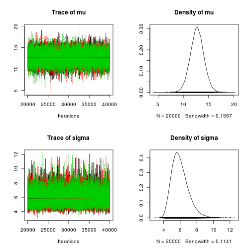
… and using summary we get credible intervals and point estimates for the parameters.
summary(mcmc_samples)
##
## Iterations = 20001:40000
## Thinning interval = 1
## Number of chains = 3
## Sample size per chain = 20000
##
## 1. Empirical mean and standard deviation for each variable,
##    plus standard error of the mean:
##
##        Mean   SD Naive SE Time-series SE
## mu    12.72 1.37  0.00558        0.00550
## sigma  5.99 1.03  0.00421        0.00639
##
## 2. Quantiles for each variable:
##
##        2.5%   25%   50%   75% 97.5%
## mu    10.03 11.83 12.72 13.60 15.40
## sigma  4.38  5.27  5.86  6.57  8.39
Method 2: STAN
STAN is a fairly new program that works in a similar way to JAGS and BUGS. You write your model in STAN’s modeling language, STAN compiles your model and generates MCMC samples that you can use for further analysis in R. All this can be done from within R using the
rstan package. One way that STAN differs from JAGS is that STAN compiles the model down to a C++ program which uses the No-U-Turn sampler to generate MCMC samples from the model. STAN’s modeling language is also a different, requiring all variables and parameters to be explicitly declared and insisting on every line ending with ;. A good introduction to STAN and rstan can be found on
STAN’s wiki page. The following R code specifies the model and runs it for 20000 MCMC samples:
library(rstan)

# The model specification
model_string <- "
data {
  int<lower=0> N;
  real y[N];
}

parameters {
  real mu;
  real<lower=0> sigma;
}
model{
  y ~ normal(mu, sigma);
  mu ~ normal(0, 100);
  sigma ~ lognormal(0, 4);
}"

# Running the model
mcmc_samples <- stan(model_code=model_string, data=list(N=length(y), y=y), pars=c("mu", "sigma"), chains=3, iter=30000, warmup=10000)
Another difference from JAGS, noticeable in the model definition above, is that STAN (in line with R) has vectorized functions. That is, what had to be written as…
for (i in y:length(y)) {
    y[i] ~ dnorm(mu, sigma)
}
… in JAGS can now simplified in STAN as:
y ~ normal(mu, sigma)
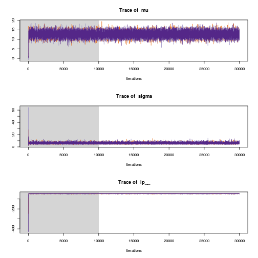
After running the model in STAN we can now inspect the trace plots…
traceplot(mcmc_samples)
… and the parameter distributions.
plot(mcmc_samples)
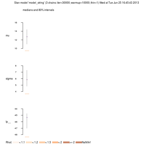
By writing the variable holding the MCMC results in the terminal we get point estimates and credible intervals.
mcmc_samples
## Inference for Stan model: model_string.
## 3 chains, each with iter=30000; warmup=10000; thin=1;
## post-warmup draws per chain=20000, total post-warmup draws=60000.
##
##        mean se_mean  sd  2.5%   25%   50%   75% 97.5% n_eff Rhat
## mu     12.7       0 1.4  10.0  11.8  12.7  13.6  15.4 25754    1
## sigma   6.0       0 1.0   4.4   5.3   5.8   6.5   8.3 25094    1
## lp__  -45.7       0 1.0 -48.4 -46.0 -45.3 -44.9 -44.6 17964    1
##
## Samples were drawn using NUTS2 at Tue Jun 25 16:45:43 2013.
## For each parameter, n_eff is a crude measure of effective sample size,
## and Rhat is the potential scale reduction factor on split chains (at
## convergence, Rhat=1).
Method 3: LaplacesDemon
Update: LaplaceDemon is unfortunately gone since mid July 2015, both the web page and the GitHub account has been removed. I’ve tried to contact the author, but has gotten no response. The last version of LaplaceDemon is now available here, but as the author has “disappeared” the future of the package is uncertain.
LaplacesDemon seems to be a rather unknown R package (I’ve found very few mentions of it on R-bloggers for example) which helps you run Bayesian models using only R. LaplacesDemon implements a plethora of different MCMC methods and has great documentation available on www.bayesian-inference.com. As opposed to JAGS and STAN there is no modeling language but instead you have to craft your own likelihood function using R. The downside of this is that your model perhaps won’t look as pretty as in JAGS but the upside is that you can be much more flexible in what constructs and probability distributions you use. Specifying and running the model using the exotic Hit-and-Run Metropolis (HARM) algorithm looks like the following:
library(LaplacesDemon)

# The model specification
model <- function(parm, data) {
    mu <- parm[1]
    sigma <- exp(parm[2])
    log_lik <- sum(dnorm(data$y, mu, sigma, log = T))
    post_lik <- log_lik + dnorm(mu, 0, 100, log = T) + dlnorm(sigma, 0, 4, log = T)
    # This list is returned and has to follow a the format specified by
    # LaplacesDemon.
    list(LP = post_lik, Dev = -2 * log_lik, Monitor = c(post_lik, sigma), yhat = NA,
        parm = parm)
}

# Running the model
data_list <- list(N = length(y), y = y, mon.names = c("post_lik", "sigma"),
    parm.names = c("mu", "log.sigma"))
mcmc_samples <- LaplacesDemon(Model = model, Data = data_list, Iterations = 30000,
    Algorithm = "HARM", Thinning = 1, Specs = list(alpha.star = 0.234))
As far as I’ve understand there is no special mechanism for keeping the parameters inside a bounded range, therefore the SD is sampled on the log-scale and then exponentiated to make sure is always positive.
The trace plots and distributions of MCMC samples can then be plotted…
plot(mcmc_samples, BurnIn = 10000, data_list)
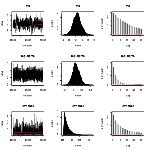
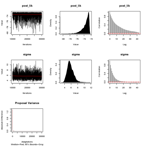
… and by Consorting with Laplace’s Demon we get a long list of info including point estimates, credible intervals and MCMC diagnostics.
Consort(mcmc_samples)
##
## #############################################################
## # Consort with Laplace's Demon                              #
## #############################################################
## Call:
## LaplacesDemon(Model = model, Data = data_list, Iterations = 30000,
##     Thinning = 1, Algorithm = "HARM", Specs = list(alpha.star = 0.234))
##
## Acceptance Rate: 0.2286
## Adaptive: 30001
## Algorithm: Hit-And-Run Metropolis
## Covariance Matrix: (NOT SHOWN HERE; diagonal shown instead)
##        mu log.sigma
##   1.86858   0.02659
##
## Covariance (Diagonal) History: (NOT SHOWN HERE)
## Deviance Information Criterion (DIC):
##          All Stationary
## Dbar 127.887    127.887
## pD     2.133      2.133
## DIC  130.021    130.021
##
## Delayed Rejection (DR): 0
## Initial Values:
##        mu log.sigma
##    12.168     1.617
##
## Iterations: 30000
## Log(Marginal Likelihood): -62.64
## Minutes of run-time: 0.1
## Model: (NOT SHOWN HERE)
## Monitor: (NOT SHOWN HERE)
## Parameters (Number of): 2
## Periodicity: 30001
## Posterior1: (NOT SHOWN HERE)
## Posterior2: (NOT SHOWN HERE)
## Recommended Burn-In of Thinned Samples: 0
## Recommended Burn-In of Un-thinned Samples: 0
## Recommended Thinning: 44
## Status is displayed every 1000 iterations
## Summary1: (SHOWN BELOW)
## Summary2: (SHOWN BELOW)
## Thinned Samples: 30000
## Thinning: 1
##
##
## Summary of All Samples
##              Mean     SD     MCSE    ESS      LB  Median      UB
## mu         12.612 1.3670 0.075629  472.6   9.911  12.613  15.378
## log.sigma   1.748 0.1631 0.004211 3142.5   1.447   1.738   2.085
## Deviance  127.887 2.0656 0.089109  964.0 125.834 127.213 133.392
## post_lik  -73.626 1.0716 0.046804  924.5 -76.459 -73.281 -72.557
## sigma       5.822 0.9775 0.025653 3102.8   4.250   5.688   8.041
##
##
## Summary of Stationary Samples
##              Mean     SD     MCSE    ESS      LB  Median      UB
## mu         12.612 1.3670 0.075629  472.6   9.911  12.613  15.378
## log.sigma   1.748 0.1631 0.004211 3142.5   1.447   1.738   2.085
## Deviance  127.887 2.0656 0.089109  964.0 125.834 127.213 133.392
## post_lik  -73.626 1.0716 0.046804  924.5 -76.459 -73.281 -72.557
## sigma       5.822 0.9775 0.025653 3102.8   4.250   5.688   8.041
##
## Demonic Suggestion
##
## Due to the combination of the following conditions,
##
## 1. Hit-And-Run Metropolis
## 2. The acceptance rate (0.2286) is within the interval [0.15,0.5].
## 3. Each target MCSE is < 6.27% of its marginal posterior
##    standard deviation.
## 4. Each target distribution has an effective sample size (ESS)
##    of at least 100.
## 5. Each target distribution became stationary by
##    1 iteration.
##
## Laplace's Demon has been appeased, and suggests
## the marginal posterior samples should be plotted
## and subjected to any other MCMC diagnostic deemed
## fit before using these samples for inference.
##
## Laplace's Demon is finished consorting.
Comparison of the Three Methods
Concluding this little exercise I thought I’d point out what I feel are some pros and cons of the three methods.
- JAGS
- + Mature program, lots of documentation and examples (for example, the great BUGS book).
- + Nice modeling language, it is almost possible to enter the likelihood specification verbatim.
- + Takes care of the sampling for you (in the best case).
- - It is difficult to use probability distributions not included in JAGS.
- - You're stuck with Gibbs sampling for better and for worse.
- STAN
- + An expressive modeling language similar to JAGS.
- + An active and supportive community (Especially the mailing lists).
- + Compiling down to C++ should result in efficient sampling.
- + The No-U-Turn sampler requires no configuration.
- + Can also do optimization (for example, maximum likelihood estimation)
- - The modeling language requires a bit more bookkeeping than JAGS' (for example, why all the `;` ?).
- - Compiling down to C++ takes some time (> 30 s on my Dell Vostro 3700)
- - It is difficult to use probability distributions not included in STAN (but easier than in JAGS)
- - No direct support for discrete parameters.
- LaplacesDemon
- + Relies only on R.
- + Easy to use any probability distribution implemented in R.
- + Good documentation.
- + Lots of different MCMC methods to try.
- - No fancy modeling language, the likelihood has to be specified using an R function.
- - No large user community.
- - You have to select and configure the MCMC sampling yourself.
- - As everything is implemented in R the sampling might be slower that in JAGS and STAN.