Update: This series of posts are now also available as a technical report:
Bååth, R. (2015), Modeling Match Results in Soccer using a Hierarchical Bayesian Poisson Model. LUCS Minor, 18. (ISSN 1104-1609) ( pdf)

This is a slightly modified version of my submission to the UseR 2013 Data Analysis Contest which I had the fortune of winning :) The purpose of the contest was to do something interesting with a dataset consisting of the match results from the last five seasons of La Liga, the premium Spanish football (aka soccer) league. In total there were 1900 rows in the dataset each with information regarding which was the home and away team, what these teams scored and what season it was. I decided to develop a Bayesian model of the distribution of the end scores. Here we go…

Ok, first I should come clean and admit that I know nothing about football. Sure, I’ve watched Sweden loose to Germany in the World Cup a couple of times, but that’s it. Never the less, here I will show an attempt to to model the goal outcomes in the La Liga data set provided as part of the UseR 2013 data analysis contest. My goal is not only to model the outcomes of matches in the data set but also to be able to (a) calculate the odds for possible goal outcomes of future matches and (b) to produce a credible ranking of the teams. The model I will be developing is a Bayesian hierarchical model where the goal outcomes will be assumed to be distributed according to a Poisson distribution. I will focus more on showing all the cool things you can easily calculate in R when you have a fully specified Bayesian Model and focus less on model comparison and trying to find the model with highest predictive accuracy (even though I believe my model is pretty good). I really would like to see somebody try to do a similar analysis in SPSS (which most people uses in my field, psychology). It would be a pain!

This post assumes some familiarity with Bayesian modeling and Markov chain Monte Carlo. If you’re not into Bayesian statistics you’re missing out on something really great and a good way to get started is by reading the excellent Doing Bayesian Data Analysis by John Kruschke. The tools I will be using is R (of course) with the model implemented in JAGS called from R using the rjags package. For plotting the result of the MCMC samples generated by JAGS I’ll use the coda package, the mcmcplots package, and the plotPost function courtesy of John Kruschke. For data manipulation I used the plyr and stringr packages and for general plotting I used ggplot2. This report was written in Rstudio using knitr and xtable.

I start by loading libraries, reading in the data and preprocessing it for JAGS. The last 50 matches have unknown outcomes and I create a new data frame d holding only matches with known outcomes. I will come back to the unknown outcomes later when it is time to use my model for prediction.

library(rjags)
library(coda)
library(mcmcplots)
library(stringr)
library(plyr)
library(xtable)
source("plotPost.R")
set.seed(12345)  # for reproducibility

load("laliga.RData")

# -1 = Away win, 0 = Draw, 1 = Home win
laliga$MatchResult <- sign(laliga$HomeGoals - laliga$AwayGoals)

# Creating a data frame d with only the complete match results
d <- na.omit(laliga)
teams <- unique(c(d$HomeTeam, d$AwayTeam))
seasons <- unique(d$Season)

# A list for JAGS with the data from d where the strings are coded as
# integers
data_list <- list(HomeGoals = d$HomeGoals, AwayGoals = d$AwayGoals, HomeTeam = as.numeric(factor(d$HomeTeam, 
    levels = teams)), AwayTeam = as.numeric(factor(d$AwayTeam, levels = teams)), 
    Season = as.numeric(factor(d$Season, levels = seasons)), n_teams = length(teams), 
    n_games = nrow(d), n_seasons = length(seasons))

# Convenience function to generate the type of column names Jags outputs.
col_name <- function(name, ...) {
    paste0(name, "[", paste(..., sep = ","), "]")
}

Modeling Match Results: Iteration 1

How are the number of goals for each team in a football match distributed? Well, let’s start by assuming that all football matches are roughly equally long, that both teams have many chances at making a goal and that each team have the same probability of making a goal each goal chance. Given these assumptions the distribution of the number of goals for each team should be well captured by a Poisson distribution. A quick and dirty comparison between the actual distribution of the number of scored goals and a Poisson distribution having the same mean number of scored goals support this notion.

par(mfcol = c(2, 1), mar = rep(2.2, 4))
hist(c(d$AwayGoals, d$HomeGoals), xlim = c(-0.5, 8), breaks = -1:9 + 0.5, main = "Distribution of the number of goals\nscored by a team in a match.")
mean_goals <- mean(c(d$AwayGoals, d$HomeGoals))
hist(rpois(9999, mean_goals), xlim = c(-0.5, 8), breaks = -1:9 + 0.5, main = "Random draw from a Poisson distribution with\nthe same mean as the distribution above.")

All teams aren’t equally good (otherwise Sweden would actually win the world cup now and then) and it will be assumed that all teams have a latent skill variable and the skill of a team minus the skill of the opposing team defines the predicted outcome of a game. As the number of goals are assumed to be Poisson distributed it is natural that the skills of the teams are on the log scale of the mean of the distribution. The distribution of the number of goals for team $i$ when facing team $j$ is then

$$Goals \sim \text{Poisson}(\lambda)$$

$$\log(\lambda) = \text{baseline} + \text{skill}_i - \text{skill}_j$$

where baseline is the log average number of goals when both teams are equally good. The goal outcome of a match between home team $i$ and away team $j$ is modeled as:

$$HomeGoals_{i,j} \sim \text{Poison}(\lambda_{\text{home},i,j})$$

$$AwayGoals_{i,j} \sim \text{Poison}(\lambda_{\text{away},i,j})$$

$$\log(\lambda_{\text{home},i,j}) = \text{baseline} + \text{skill}_i - \text{skill}_j$$

$$\log(\lambda_{\text{away},i,j}) = \text{baseline} + \text{skill}_j - \text{skill}_i$$

Add some priors to that and you’ve got a Bayesian model going! I set the prior distributions over the baseline and the skill of all $n$ teams to:

$$\text{baseline} \sim \text{Normal}(0, 4^2)$$

$$\text{skill}{1 \ldots n} \sim \text{Normal}(\mu\text{teams}, \sigma_{\text{teams}}^2)$$

$$\mu_\text{teams} \sim \text{Normal}(0, 4^2)$$

$$\sigma_\text{teams} \sim \text{Uniform}(0, 3)$$

Since I know nothing about football these priors are made very vague. For example, the prior on the baseline have a SD of 4 but since this is on the log scale of the mean number of goals it corresponds to one SD from the mean $0$ covering the range of $[0.02, 54.6]$ goals. A very wide prior indeed.

Turning this into a JAGS model requires some minor adjustments. The model have to loop over all the match results, which adds some for-loops. JAGS parameterizes the normal distribution with precision (the reciprocal of the variance) instead of variance so the hyper priors have to be converted. Finally I have to “anchor” the skill of one team to a constant otherwise the mean skill can drift away freely. Doing these adjustments results in the following model description:

m1_string <- "model {
for(i in 1:n_games) {
  HomeGoals[i] ~ dpois(lambda_home[HomeTeam[i],AwayTeam[i]])
  AwayGoals[i] ~ dpois(lambda_away[HomeTeam[i],AwayTeam[i]])
}

for(home_i in 1:n_teams) {
  for(away_i in 1:n_teams) {
    lambda_home[home_i, away_i] <- exp(baseline + skill[home_i] - skill[away_i])
    lambda_away[home_i, away_i] <- exp(baseline + skill[away_i] - skill[home_i])
  }
}

skill[1] <- 0
for(j in 2:n_teams) {
  skill[j] ~ dnorm(group_skill, group_tau)
}  

group_skill ~ dnorm(0, 0.0625)
group_tau <- 1 / pow(group_sigma, 2)
group_sigma ~ dunif(0, 3)
baseline ~ dnorm(0, 0.0625)
}"

I can then run this model directly from R using rjags and the handy textConnection function. This takes a couple of minutes on my computer, roughly enough for a coffee break.

# Compiling model 1
m1 <- jags.model(textConnection(m1_string), data = data_list, n.chains = 3, 
    n.adapt = 5000)
# Burning some samples on the altar of the MCMC god
update(m1, 5000)
# Generating MCMC samples
s1 <- coda.samples(m1, variable.names = c("baseline", "skill", "group_skill", 
    "group_sigma"), n.iter = 10000, thin = 2)
# Merging the three MCMC chains into one matrix
ms1 <- as.matrix(s1)

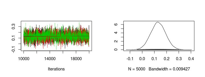
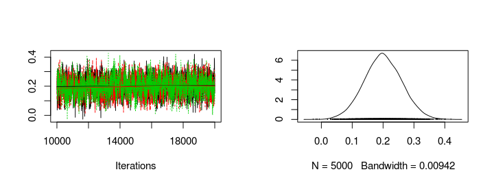
Using the generated MCMC samples I can now look at the credible skill values of any team. Let’s look at the trace plot and the distribution of the skill parameters for FC Sevilla and FC Valencia.

plot(s1[, col_name("skill", which(teams == "FC Sevilla"))])

plot(s1[, col_name("skill", which(teams == "FC Valencia"))])

Seems like Sevilla and Valencia have similar skill with Valencia being slightly better. Using the MCMC samples it is not only possible to look at the distribution of parameter values but it is also straight forward to simulate matches between teams and look at the credible distribution of number of goals scored and the probability of a win for the home team, a win for the away team or a draw. The following functions simulates matches with one team as home team and one team as away team and plots the predicted result together with the actual outcomes of any matches in the laliga data set.

# Plots histograms over home_goals, away_goals, the difference in goals
# and a barplot over match results.
plot_goals <- function(home_goals, away_goals) {
    n_matches <- length(home_goals)
    goal_diff <- home_goals - away_goals
    match_result <- ifelse(goal_diff < 0, "away_win", ifelse(goal_diff > 0, 
        "home_win", "equal"))
    hist(home_goals, xlim = c(-0.5, 10), breaks = (0:100) - 0.5)
    hist(away_goals, xlim = c(-0.5, 10), breaks = (0:100) - 0.5)
    hist(goal_diff, xlim = c(-6, 6), breaks = (-100:100) - 0.5)
    barplot(table(match_result)/n_matches, ylim = c(0, 1))
}


plot_pred_comp1 <- function(home_team, away_team, ms) {
    # Simulates and plots game goals scores using the MCMC samples from the m1
    # model.
    par(mfrow = c(2, 4))
    baseline <- ms[, "baseline"]
    home_skill <- ms[, col_name("skill", which(teams == home_team))]
    away_skill <- ms[, col_name("skill", which(teams == away_team))]
    home_goals <- rpois(nrow(ms), exp(baseline + home_skill - away_skill))
    away_goals <- rpois(nrow(ms), exp(baseline + away_skill - home_skill))
    plot_goals(home_goals, away_goals)
    # Plots the actual distribution of goals between the two teams
    home_goals <- d$HomeGoals[d$HomeTeam == home_team & d$AwayTeam == away_team]
    away_goals <- d$AwayGoals[d$HomeTeam == home_team & d$AwayTeam == away_team]
    plot_goals(home_goals, away_goals)
}

Let’s look at Valencia (home team) vs. Sevilla (away team). The graph below shows the simulation on the first row and the historical data on the second row.

plot_pred_comp1("FC Valencia", "FC Sevilla", ms1)

The simulated data fits the historical data reasonably well and both the historical data and the simulation show that Valencia would win with a slightly higher probability that Sevilla. Let’s swap places and let Sevilla be the home team and Valencia be the away team.

plot_pred_comp1("FC Sevilla", "FC Valencia", ms1)

Here we discover a problem with the current model. While the simulated data looks the same, except that the home team and the away team swapped places, the historical data now shows that Sevilla often wins against Valencia when being the home team. Our model doesn’t predict this because it doesn’t considers the advantage of being the home team. This is fortunately easy to fix as I will show in part two of Modeling Match Results in La Liga Using a Hierarchical Bayesian Poisson Model.