Except for maybe the t test, a contender for the title “most used and abused statistical test” is Pearson’s correlation test. Whenever someone wants to check if two variables relate somehow it is a safe bet (at least in psychology) that the first thing to be tested is the strength of a Pearson’s correlation. Only if that doesn’t work a more sophisticated analysis is attempted (“That p-value is still to big, maybe a mixed models logistic regression will make it smaller…”). One reason for this is that the Pearson’s correlation test is conceptually quite simple and have assumption that makes it applicable in many situations (but it is definitely also used in many situations where underlying assumption are violated).
Since I’ve converted to “Bayesianism” I’ve been trying to figure out what Bayesian analyses correspond to the classical analyses. For t tests, chi-square tests and Anovas I’ve found Bayesian versions that, at least conceptually, are testing the same thing. Here are links to Bayesian versions of the t test, a chi-square test and an Anova, if you’re interested. But for some reason I’ve never encountered a discussion of what a Pearson’s correlation test would correspond to in a Bayesian context. Maybe this is because regression modeling often can fill the same roll as correlation testing (quantifying relations between continuous variables) or perhaps I’ve been looking in the wrong places.
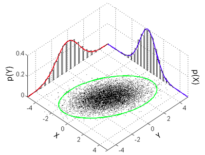
The aim of this post is to explain how one can run the Bayesian counterpart of Pearson’s correlation test using R and JAGS. The model that a classical Pearson’s correlation test assumes is that the data follows a bivariate normal distribution. That is, if we have a list of pairs of data points then the and the are each assumed to be normally distributed with a possible linear dependency between them. This dependency is quantified by the correlation parameter which is what we want to estimate in a correlation analysis. A good visualization of a bivariate normal distribution with can be found on the the wikipedia page on the multivariate normal distribution :

We will assume the same model and our Bayesian correlation analysis then reduces to estimating the parameters of a bivariate normal distribution given some data. One problem is that the bivariate normal distribution and, more general, the multivariate normal distribution isn’t parameterized using , that is, we cannot estimate directly. The bivariate normal is parameterized using and the means of the two marginal distributions (the red and blue normal distribution in the graph above) and a covariance matrix which defines and , the variances of the two marginal distributions, and the covariance, how much the marginal distributions vary together. So the covariance is another measure of how much two variables vary together and the covariance corresponding to a correlation of can be calculated as . So here is the model we want to estimate:
Add some flat priors on this (which could, of course, be made more informative) and we’re ready to roll:
Implementation
So, how to implement this model? I’m going to do it with R and the JAGS sampler interfaced with R using the
rjags package. First I’m going to simulate some data with a correlation of 0.7 to test the model with.
library(rjags)
library(mvtnorm) # to generate correlated data with rmvnorm.
library(car) # To plot the estimated bivariate normal distribution.
set.seed(31415)

mu <- c(10, 30)
sigma <- c(20, 40)
rho <- -0.7
cov_mat <- rbind(c(     sigma[1]^2       , sigma[1]*sigma[2]*rho ),
                 c( sigma[1]*sigma[2]*rho,      sigma[2]^2       ))
x <- rmvnorm(30, mu, cov_mat)
plot(x, xlim=c(-125, 125), ylim=c(-100, 150))

The simulated data looks quite correlated and a classical Pearson’s correlation test confirms this:
cor.test(x[, 1], x[, 2])
##
## 	Pearson's product-moment correlation
##
## data:  x[, 1] and x[, 2]
## t = -6.6, df = 28, p-value = 3.704e-07
## alternative hypothesis: true correlation is not equal to 0
## 95 percent confidence interval:
##  -0.8902 -0.5841
## sample estimates:
##     cor
## -0.7802
The JAGS model below implements the bivariate normal model described above. One difference is that JAGS parameterizes the normal and multivariate normal distributions with precision instead of standard deviation or variance. The precision is the inverse of the variance so in order to use a covariance matrix as a parameter to dmnorm we have to inverse it first using the inverse function.
model_string <- "
  model {
    for(i in 1:n) {
      x[i,1:2] ~ dmnorm(mu[], prec[ , ])
    }

    # Constructing the covariance matrix and the corresponding precision matrix.
    prec[1:2,1:2] <- inverse(cov[,])
    cov[1,1] <- sigma[1] * sigma[1]
    cov[1,2] <- sigma[1] * sigma[2] * rho
    cov[2,1] <- sigma[1] * sigma[2] * rho
    cov[2,2] <- sigma[2] * sigma[2]

    # Uninformative priors on all parameters which could, of course, be made more informative.
    sigma[1] ~ dunif(0, 1000)
    sigma[2] ~ dunif(0, 1000)
    rho ~ dunif(-1, 1)
    mu[1] ~ dnorm(0, 0.001)
    mu[2] ~ dnorm(0, 0.001)

    # Generate random draws from the estimated bivariate normal distribution
    x_rand ~ dmnorm(mu[], prec[ , ])
  }
"
Update: Note that while the priors defined in model_string are relatively uninformative for my data, they are not necessary uninformative in general. For example, the priors above considers a value of mu[1] as large as 10000 extremely improbable and a value of sigma[1] above 1000 impossible. An example of more vague priors would for example be:
sigma[1] ~ dunif(0, 100000)
sigma[2] ~ dunif(0, 100000)
mu[1] ~ dnorm(0, 0.000001)
mu[2] ~ dnorm(0, 0.000001)
If you decide to use the model above, it is advisable that you think about what could be reasonable priors. End of update
An extra feature is that the model above generates random samples (x_rand) from the estimated bivariate normal distribution. These samples can be compared to the actual data in order to get a sense of how well the model fits the data. Now let’s use JAGS to sample from this model. I’m using the textConnection trick (described
here) in order to run the model without having to first save the model string to a file.
data_list = list(x = x, n = nrow(x))
# Use classical estimates of the parameters as initial values
inits_list = list(mu = c(mean(x[, 1]), mean(x[, 2])),
                  rho = cor(x[, 1], x[, 2]),
                  sigma = c(sd(x[, 1]), sd(x[, 1])))
jags_model <- jags.model(textConnection(model_string), data = data_list, inits = inits_list,
    n.adapt = 500, n.chains = 3, quiet = T)
update(jags_model, 500)
mcmc_samples <- coda.samples(jags_model, c("mu", "rho", "sigma", "x_rand"),
    n.iter = 5000)
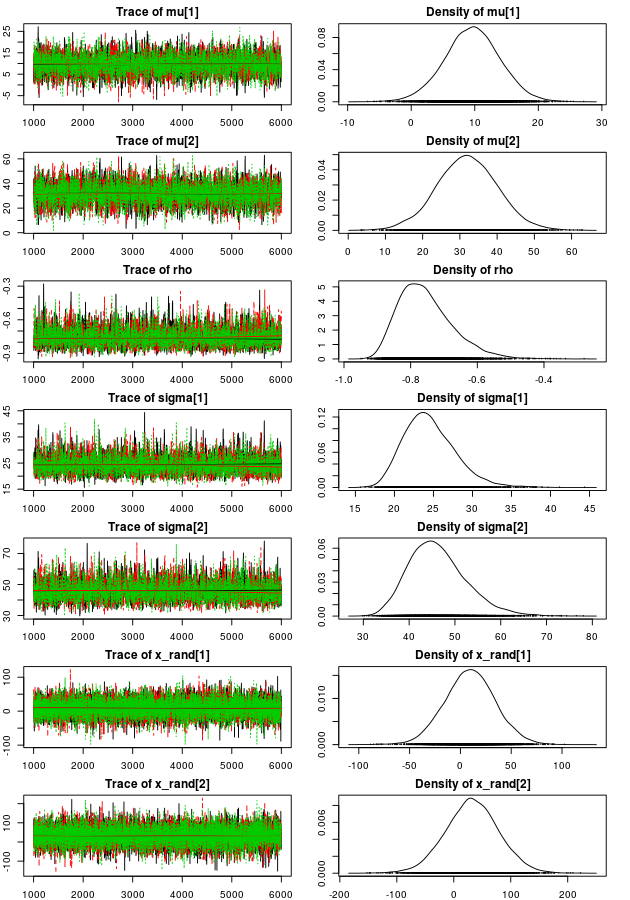
Now let’s plot trace plots and density plots of the MCMC parameter estimates:
par(mfrow = c(7, 2), mar = rep(2, 4))
plot(mcmc_samples, auto.layout = FALSE)

The trace plots look sufficiently furry and stationary and looking at the density plots it looks like the model have captured the “true” parameters well (those used when we created the data). Looking at point estimates and credible intervals confirms this:
summary(mcmc_samples)
##
## Iterations = 1001:6000
## Thinning interval = 1
## Number of chains = 3
## Sample size per chain = 5000
##
## 1. Empirical mean and standard deviation for each variable,
##    plus standard error of the mean:
##
##             Mean      SD Naive SE Time-series SE
## mu[1]      9.621  4.3713 0.035692        0.07107
## mu[2]     31.988  8.1653 0.066669        0.13381
## rho       -0.755  0.0816 0.000666        0.00142
## sigma[1]  24.531  3.3368 0.027245        0.05816
## sigma[2]  46.230  6.2924 0.051377        0.11245
## x_rand[1]  9.513 24.9313 0.203563        0.21112
## x_rand[2] 32.353 47.1290 0.384806        0.39614
##
## 2. Quantiles for each variable:
##
##              2.5%    25%    50%    75%   97.5%
## mu[1]       0.970  6.779  9.640 12.485  18.178
## mu[2]      15.671 26.551 31.969 37.371  48.264
## rho        -0.881 -0.814 -0.766 -0.708  -0.564
## sigma[1]   19.042 22.181 24.174 26.517  32.003
## sigma[2]   35.662 41.750 45.583 49.980  60.509
## x_rand[1] -39.002 -6.852  9.658 25.964  58.649
## x_rand[2] -60.836  1.619 32.223 63.050 125.009
The median of the rho parameter is -0.76 (95% CI: [-0.88, -0.55]) close to the true parameter value -0.7. Even if this is not that strange, we did use a bivariate normal distribution both to generate and model the data, it is nice when things work out :) Now let’s calculate the probability that there actually is a negative correlation.
samples_mat <- as.matrix(mcmc_samples)
mean(samples_mat[, "rho"] < 0)
## [1] 1
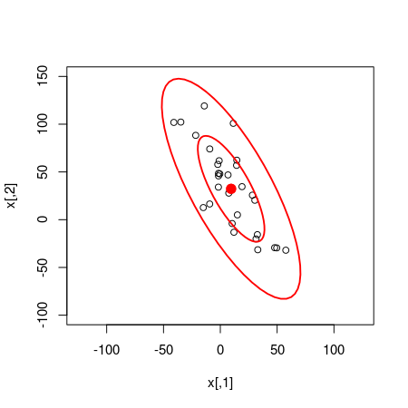
Given the model and the data it seems like the probability that there is a negative correlation is 100%. Accounting for the MCMC error I think it is fair to downgrade this probability to at least 99.9%. We can also use the random samples from the bivariate normal distribution estimated by the model to compare how well the model fits the data. The following code plots the original data with two superimposed ellipses where the inner ellipse covers 50% of the density of the distribution and the outer ellipse covers 95%.
plot(x, xlim = c(-125, 125), ylim = c(-100, 150))
dataEllipse(samples_mat[, c("x_rand[1]", "x_rand[2]")], levels = c(0.5, 0.95),
    plot.points = FALSE)

Quite a good fit!
Update: If you are more of a Python person, check out Philipp Singer’s Bayesian Correlation with PyMC, which implements the model above in Python.
Analysis of Some “Real” Data
So let’s use this model on some real data. The data.frame below contains the names, weights in kg and finishing times for all participants of the men’s 100 m semi-finals in the 2013 World Championships in Athletics. Well, those I could find the weights of anyway…
d <- data.frame(runner = c("Usain Bolt", "Justin Gatlin", "Nesta Carter", "Kemar Bailey-Cole",
    "Nickel Ashmeade", "Mike Rodgers", "Christophe Lemaitre", "James Dasaolu",
    "Zhang Peimeng", "Jimmy Vicaut", "Keston Bledman", "Churandy Martina", "Dwain Chambers",
    "Jason Rogers", "Antoine Adams", "Anaso Jobodwana", "Richard Thompson",
    "Gavin Smellie", "Ramon Gittens", "Harry Aikines-Aryeetey"), time = c(9.92,
    9.94, 9.97, 9.93, 9.9, 9.93, 10, 9.97, 10, 10.01, 10.08, 10.09, 10.15, 10.15,
    10.17, 10.17, 10.19, 10.3, 10.31, 10.34), weight = c(94, 79, 78, 83, 77,
    76, 74, 87, 86, 83, 75, 74, 92, 69, 79, 71, 80, 80, 77, 87))
d
##                    runner  time weight
## 1              Usain Bolt  9.92     94
## 2           Justin Gatlin  9.94     79
## 3            Nesta Carter  9.97     78
## 4       Kemar Bailey-Cole  9.93     83
## 5         Nickel Ashmeade  9.90     77
## 6            Mike Rodgers  9.93     76
## 7     Christophe Lemaitre 10.00     74
## 8           James Dasaolu  9.97     87
## 9           Zhang Peimeng 10.00     86
## 10           Jimmy Vicaut 10.01     83
## 11         Keston Bledman 10.08     75
## 12       Churandy Martina 10.09     74
## 13         Dwain Chambers 10.15     92
## 14           Jason Rogers 10.15     69
## 15          Antoine Adams 10.17     79
## 16        Anaso Jobodwana 10.17     71
## 17       Richard Thompson 10.19     80
## 18          Gavin Smellie 10.30     80
## 19          Ramon Gittens 10.31     77
## 20 Harry Aikines-Aryeetey 10.34     87
So, I know nothing about running (and I’m not sure this is a very representative data set…) but my hypothesis is that there should be a positive correlation between weight and finishing time. That is, the more you weigh the slower you run. Sounds like logic, right? Let’s look at the data…
plot(d$time, d$weight)

At a first glance it seems like my hypothesis is not supported by the data. I wonder what our model has to say about that?
data_list = list(x = d[, c("time", "weight")], n = nrow(d))
# Use classical estimates of the parameters as initial values
inits_list = list(mu = c(mean(d$time), mean(d$weight)), rho = cor(d$time, d$weight),
    sigma = c(sd(d$time), sd(d$weight)))
jags_model <- jags.model(textConnection(model_string), data = data_list, inits = inits_list,
    n.adapt = 500, n.chains = 3, quiet = T)
update(jags_model, 500)
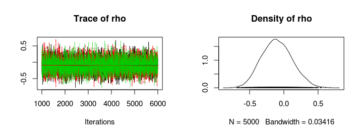
mcmc_samples <- coda.samples(jags_model, c("rho"), n.iter = 5000)
plot(mcmc_samples)

summary(mcmc_samples)
##
## Iterations = 1001:6000
## Thinning interval = 1
## Number of chains = 3
## Sample size per chain = 5000
##
## 1. Empirical mean and standard deviation for each variable,
##    plus standard error of the mean:
##
##           Mean             SD       Naive SE Time-series SE
##       -0.09905        0.22054        0.00180        0.00243
##
## 2. Quantiles for each variable:
##
##    2.5%     25%     50%     75%   97.5%
## -0.5084 -0.2548 -0.1053  0.0498  0.3455
Seems like there is no support for my hypothesis, the posterior distribution of rho is centered around zero and, if anything, there might be a tiny negative correlation. So your weight doesn’t seem to influence how fast you run (if you are a runner in the 100 m semi finals, at least).