In part one and part two of Modeling Match Results in La Liga Using a Hierarchical Bayesian Poisson Model I developed a model for the number of goals in football matches from five seasons of La Liga, the premier Spanish football league. I’m now reasonably happy with the model and want to use it to rank the teams in La Liga and to predict the outcome of future matches!
Ranking the Teams of La Liga
We’ll start by ranking the teams of La Liga using the estimated skill parameters from the 2012/2013 season. The values of the skill parameters are difficult to interpret as they are relative to the skill of the team that had its skill parameter “anchored” at zero. To put them on a more interpretable scale I’ll first zero center the skill parameters by subtracting the mean skill of all teams, I then add the home baseline and exponentiate the resulting values. These rescaled skill parameters are now on the scale of expected number of goals when playing home team. Below is a caterpillar plot of the median of the rescaled skill parameters together with the 68 % and 95 % credible intervals. The plot is ordered according to the median skill and thus also gives the ranking of the teams.
# The ranking of the teams for the 2012/13 season.
team_skill <- ms3[, str_detect(string = colnames(ms3), "skill\\[5,")]
team_skill <- (team_skill - rowMeans(team_skill)) + ms3[, "home_baseline[5]"]
team_skill <- exp(team_skill)
colnames(team_skill) <- teams
team_skill <- team_skill[, order(colMeans(team_skill), decreasing = T)]
par(mar = c(2, 0.7, 0.7, 0.7), xaxs = "i")
caterplot(team_skill, labels.loc = "above", val.lim = c(0.7, 3.8))
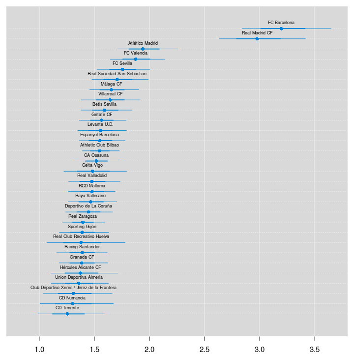
Two teams are clearly ahead of the rest, FC Barcelona and Real Madrid CF. Let’s look at the credible difference between the two teams.
plotPost(team_skill[, "FC Barcelona"] - team_skill[, "Real Madrid CF"], compVal = 0,
    xlab = "← Real Madrid     vs     Barcelona →")
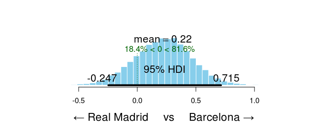
FC Barcelona is the better team with a probability of 82 % . Go Barcelona!
Predicting the End Game of La Liga 2012/2013
In the laliga data set the results of the 50 last games of the 2012/2013 season was missing. Using our model we can now both predict and simulate the outcomes of these 50 games. The R code below calculates a number of measures for each game (both the games with known and unknown outcomes):
- The mode of the simulated number of goals, that is, the most likely number of scored goals. If we were asked to bet on the number of goals in a game this is what we would use.
- The mean of the simulated number of goals, this is our best guess of the average number of goals in a game.
- The most likely match result for each game.
- A random sample from the distributions of credible home scores, away scores and match results. This is how La Liga actually could have played out in an alternative reality…
n <- nrow(ms3)
m3_pred <- sapply(1:nrow(laliga), function(i) {
  home_team <- which(teams == laliga$HomeTeam[i])
  away_team <- which(teams == laliga$AwayTeam[i])
  season <- which(seasons == laliga$Season[i])
  home_skill <- ms3[, col_name("skill", season, home_team)]
  away_skill <- ms3[, col_name("skill", season, away_team)]
  home_baseline <- ms3[, col_name("home_baseline", season)]
  away_baseline <- ms3[, col_name("away_baseline", season)]

  home_goals <- rpois(n, exp(home_baseline + home_skill - away_skill))
  away_goals <- rpois(n, exp(away_baseline + away_skill - home_skill))
  home_goals_table <- table(home_goals)
  away_goals_table <- table(away_goals)
  match_results <- sign(home_goals - away_goals)
  match_results_table <- table(match_results)

  mode_home_goal <- as.numeric(names(home_goals_table)[ which.max(home_goals_table)])
  mode_away_goal <- as.numeric(names(away_goals_table)[ which.max(away_goals_table)])
  match_result <-  as.numeric(names(match_results_table)[which.max(match_results_table)])
  rand_i <- sample(seq_along(home_goals), 1)

  c(mode_home_goal = mode_home_goal, mode_away_goal = mode_away_goal, match_result = match_result,
    mean_home_goal = mean(home_goals), mean_away_goal = mean(away_goals),
    rand_home_goal = home_goals[rand_i], rand_away_goal = away_goals[rand_i],
    rand_match_result = match_results[rand_i])
})
m3_pred <- t(m3_pred)
First let’s compare the distribution of the number of goals in the data with the predicted mode, mean and randomized number of goals for all the games (focusing on the number of goals for the home team).
First the actual distribution of the number of goals for the home teams.
hist(laliga$HomeGoals, breaks = (-1:10) + 0.5, xlim = c(-0.5, 10), main = "Distribution of the number of goals\nscored by a home team in a match.",
    xlab = "")

This next plot shows the distribution of the modes from the predicted distribution of home goals from each game. That is, what is the most probable outcome, for the home team, in each game.
hist(m3_pred[, "mode_home_goal"], breaks = (-1:10) + 0.5, xlim = c(-0.5, 10),
    main = "Distribution of predicted most\nprobable scoreby a home team in\na match.",
    xlab = "")

For almost all games the single most likely number of goals is one. Actually, if you know nothing about a La Liga game betting on one goal for the home team is 78 % of the times the best bet.
Lest instead look at the distribution of the predicted mean number of home goals in each game.
hist(m3_pred[, "mean_home_goal"], breaks = (-1:10) + 0.5, xlim = c(-0.5, 10),
    main = "Distribution of predicted mean \n score by a home team in a match.",
    xlab = "")

For most games the expected number of goals are 2. That is, even if your safest bet is one goal you would expect to see around two goals.
The distribution of the mode and the mean number of goals doesn’t look remotely like the actual number of goals. This was not to be expected, we would however expect the distribution of randomized goals (where for each match the number of goals has been randomly drawn from that match’s predicted home goal distribution) to look similar to the actual number of home goals. Looking at the histogram below, this seems to be the case.
hist(m3_pred[, "rand_home_goal"], breaks = (-1:10) + 0.5, xlim = c(-0.5, 10),
    main = "Distribution of randomly draw \n score by a home team in a match.",
    xlab = "")

We can also look at how well the model predicts the data. This should probably be done using cross validation, but as the number of effective parameters are much smaller than the number of data points a direct comparison should at least give an estimated prediction accuracy in the right ballpark.
mean(laliga$HomeGoals == m3_pred[, "mode_home_goal"], na.rm = T)
## [1] 0.3351
mean((laliga$HomeGoals - m3_pred[, "mean_home_goal"])^2, na.rm = T)
## [1] 1.452
So on average the model predicts the correct number of home goals 34 % of the time and guesses the average number of goals with a mean squared error of 1.45 . Now we’ll look at the actual and predicted match outcomes. The graph below shows the match outcomes in the data with 1 being a home win, 0 being a draw and -1 being a win for the away team.
hist(laliga$MatchResult, breaks = (-2:1) + 0.5, main = "Actual match results.",
    xlab = "")

Now looking at the most probable outcomes of the matches according to the model.
hist(m3_pred[, "match_result"], breaks = (-2:1) + 0.5, main = "Predicted match results.",
    xlab = "")

For almost all matches the safest bet is to bet on the home team. While draws are not uncommon it is never the safest bet.
As in the case with the number of home goals, the randomized match outcomes have a distribution similar to the actual match outcomes:
hist(m3_pred[, "rand_match_result"], breaks = (-2:1) + 0.5, main = "Randomized match results.",
    xlab = "")

mean(laliga$MatchResult == m3_pred[, "match_result"], na.rm = T)
## [1] 0.5627
The model predicts the correct match outcome 56 % of the time. Pretty good!
Now that we’ve checked that the model reasonably predicts the La Liga history let’s predict the La Liga endgame! The code below displays the predicted mode and mean number of goals for the endgame and the predicted winner of each game.
laliga_forecast <- laliga[is.na(laliga$HomeGoals), c("Season", "Week", "HomeTeam",
    "AwayTeam")]
m3_forecast <- m3_pred[is.na(laliga$HomeGoals), ]
laliga_forecast$mean_home_goals <- round(m3_forecast[, "mean_home_goal"], 1)
laliga_forecast$mean_away_goals <- round(m3_forecast[, "mean_away_goal"], 1)
laliga_forecast$mode_home_goals <- m3_forecast[, "mode_home_goal"]
laliga_forecast$mode_away_goals <- m3_forecast[, "mode_away_goal"]
laliga_forecast$predicted_winner <- ifelse(m3_forecast[, "match_result"] ==
    1, laliga_forecast$HomeTeam, ifelse(m3_forecast[, "match_result"] == -1,
    laliga_forecast$AwayTeam, "Draw"))

rownames(laliga_forecast) <- NULL
print(xtable(laliga_forecast, align = "cccccccccc"), type = "html")
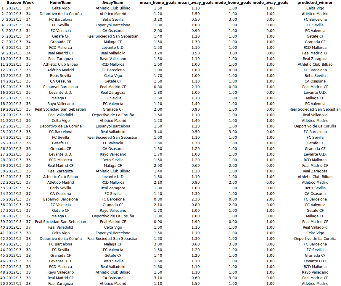
While these predictions are good if you want to bet on the likely winner they do not reflect how the actual endgame will play out, e.g., there is not a single draw in the predicted_winner column. So at last let’s look at a possible version of the La Liga endgame by displaying the simulated match results calculated earlier.
laliga_sim <- laliga[is.na(laliga$HomeGoals), c("Season", "Week", "HomeTeam",
    "AwayTeam")]
laliga_sim$home_goals <- m3_forecast[, "rand_home_goal"]
laliga_sim$away_goals <- m3_forecast[, "rand_away_goal"]
laliga_sim$winner <- ifelse(m3_forecast[, "rand_match_result"] == 1, laliga_forecast$HomeTeam,
    ifelse(m3_forecast[, "rand_match_result"] == -1, laliga_forecast$AwayTeam,
        "Draw"))

rownames(laliga_sim) <- NULL
print(xtable(laliga_sim, align = "cccccccc"), type = "html")

Now we see a number of games resulting in a draw. We also see that Málaga manages to beat Real Madrid in week 36, against all odds, even though playing as the away team. An amazing day for all Málaga fans!
Calculating the Predicted Payout for Sevilla vs Valencia, 2013-06-01
At the time when I developed this model (2013-05-28) most of the matches in the 2012/2013 season had been played and Barcelona was already the winner (and the most skilled team as predicted by my model). There were however some matches left, for example, Sevilla (home team) vs Valencia (away team) at the 1st of June, 2013. One of the powers with using Bayesian modeling and MCMC sampling is that once you have the MCMC samples of the parameters it is straight forward to calculate any quantity resulting from these estimates while still retaining the uncertainty of the parameter estimates. So let’s look at the predicted distribution of the number of goals for the Sevilla vs Valencia game and see if I can use my model to make some money. I’ll start by using the MCMC samples to calculate the distribution of the number of goals for Sevilla and Valencia.
n <- nrow(ms3)
home_team <- which(teams == "FC Sevilla")
away_team <- which(teams == "FC Valencia")
season <- which(seasons == "2012/13")
home_skill <- ms3[, col_name("skill", season, home_team)]
away_skill <- ms3[, col_name("skill", season, away_team)]
home_baseline <- ms3[, col_name("home_baseline", season)]
away_baseline <- ms3[, col_name("away_baseline", season)]

home_goals <- rpois(n, exp(home_baseline + home_skill - away_skill))
away_goals <- rpois(n, exp(away_baseline + away_skill - home_skill))
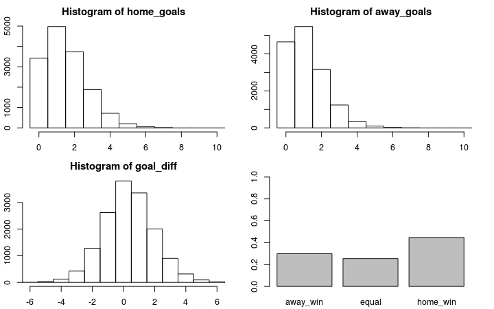
Looking at summary of these two distributions shows that it will be a close game but with a slight advantage for the home team Sevilla.
par(mfrow = c(2, 2), mar = rep(2.2, 4))
plot_goals(home_goals, away_goals)
When developing the model (2013-05-28) I got the following payouts (that is, how much would I get back if my bet was successful) for betting on the outcome of this game on the betting site www.betsson.com:
 Sevilla  Draw  Valencia
   3.2    3.35    2.15
Using my simulated distribution of the number of goals I can calculate the predicted payouts of my model.
1/c(Sevilla = mean(home_goals > away_goals), Draw = mean(home_goals == away_goals),
    Valencia = mean(home_goals < away_goals))
##  Sevilla     Draw Valencia
##    2.237    3.940    3.343
I should clearly bet on Sevilla as my model predicts a payout of 2.24 (that is, a likely win for Sevilla) while betsson.com gives me the much higher payout of 3.2. It is also possible to bet on the final goal outcome so let’s calculate what payouts my model predicts for different goal outcomes.
goals_payout <- laply(0:6, function(home_goal) {
    laply(0:6, function(away_goal) {
        1/mean(home_goals == home_goal & away_goals == away_goal)
    })
})

colnames(goals_payout) <- paste("Valencia", 0:6, sep = " - ")
rownames(goals_payout) <- paste("Sevilla", 0:6, sep = " - ")
goals_payout <- round(goals_payout, 1)
print(xtable(goals_payout, align = "cccccccc"), type = "html")
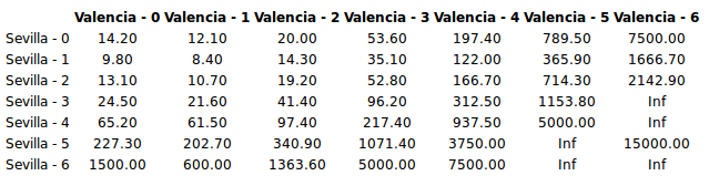
The most likely result is 1 - 1 with a predicted payout of 8.4 and betsson.com agrees with this also offering their lowest payout for this bet, 5.3. Not good enough! Looking at the payouts at bettson.com I can see that Sevilla - Valencia: 2 - 0 gives me a payout of 16.0, that’s much better than my predicted payout of 13.1. I’ll go for that!
Wrap-up
I believe my model has a lot things going for it. It is conceptually quite simple and easy to understand, implement and extend. It captures the patterns in and distribution of the data well. It allows me to easily calculate the probability of any outcome, from a game with whichever teams from any La Liga season. Want to calculate the probability that RCD Mallorca (home team) vs Málaga CF (away team) in the Season 2009/2010 would result in a draw? Easy! What’s the probability of the total number of goals in Granada CF vs Athletic Club Bilbao being a prime number? No problemo! What if Real Madrid from 2008/2009 met Barcelona from 2012/2013 in 2010/2011 and both teams had the home advantage? Well, that’s possible…
There are also a couple of things that could be improved (many which are not too hard to address).
- Currently there is assumed to be no dependency between the goal distributions of the home and away teams, but this might not be realistic. Maybe if one team have scored more goals the other team “looses steam” (a negative correlation between the teams’ scores) or instead maybe the other team tries harder (a positive correlation). Such dependencies could maybe be added to the model using copulas.
- One of the advantages of Bayesian statistics is the possibility to used informative priors. As I have no knowledge of football I’ve been using vague priors but with the help of a more knowledgeable football fan the model could be given more informative priors.
- The predictive performance of the model has not been as thoroughly examined and this could be remedied with a healthy dose of cross validation.
- The graphs could be much prettier, but this submission was for the data analysis contest of UseR 2014 not the data visualtization contest, so…
So this has been a journey, like a pirate on the open sea I’ve been sailing on a sea of data salvaging and looting whatever I could with the power of JAGS and R (read ARRRHHH!). And still without knowing anything about football I can now log onto bettson.com and with confidence bet 100 Swedish kronas on Sevilla next week winning with 2 - 0 against Valencia. ¡Adelante Sevilla!
Edit: At time of writing the match between Sevilla and Valencia has been played and my bet was a partial success. I betted 50 sek on Sevilla winning the game and 50 sek on Sevilla winning with 2 - 0. Against the (betsson.com) odds Sevilla did win the game, which gave me $50 \cdot 3.2=160$ sek, but unfortunately for me not with 2-0 but with 4-3. In total I betted 100 sek and got 160 sek back so good enough for me :)