So in the last post I showed how to run the Bayesian counterpart of Pearson’s correlation test by estimating the parameters of a bivariate normal distribution. A problem with assuming normality is that the normal distribution isn’t robust against outliers. Let’s see what happens if we take the data from the last post with the finishing times and weights of the runners in the men’s 100 m semi-finals in the 2013 World Championships in Athletics and introduce an outlier. This is how the original data looks:
d
##                    runner  time weight
## 1              Usain Bolt  9.92     94
## 2           Justin Gatlin  9.94     79
## 3            Nesta Carter  9.97     78
## 4       Kemar Bailey-Cole  9.93     83
## 5         Nickel Ashmeade  9.90     77
## 6            Mike Rodgers  9.93     76
## 7     Christophe Lemaitre 10.00     74
## 8           James Dasaolu  9.97     87
## 9           Zhang Peimeng 10.00     86
## 10           Jimmy Vicaut 10.01     83
## 11         Keston Bledman 10.08     75
## 12       Churandy Martina 10.09     74
## 13         Dwain Chambers 10.15     92
## 14           Jason Rogers 10.15     69
## 15          Antoine Adams 10.17     79
## 16        Anaso Jobodwana 10.17     71
## 17       Richard Thompson 10.19     80
## 18          Gavin Smellie 10.30     80
## 19          Ramon Gittens 10.31     77
## 20 Harry Aikines-Aryeetey 10.34     87
What if Usain Bolt had eaten mutant cheese burgers both gaining in weight and ability to run faster?
d[d$runner == "Usain Bolt", c("time", "weight")] <- c(9.5, 115)
plot(d$time, d$weight)

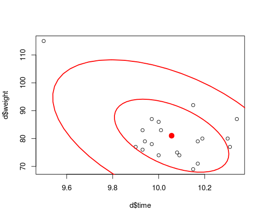
Usain Bolt now looks like a real outlier, and he is, he’s not representative of the majority of runners that are not eating mutant cheeseburgers and that we would like to make inferences about. How does this single outlier influence the estimated correlation between finishing time and weight? Let’s rerun the correlation analysis from the last post and compare:
data_list = list(x = d[, c("time", "weight")], n = nrow(d))
# Use classical estimates of the parameters as initial values
inits_list = list(mu = c(mean(d$time), mean(d$weight)), rho = cor(d$time, d$weight),
    sigma = c(sd(d$time), sd(d$weight)))
jags_model <- jags.model(textConnection(model_string), data = data_list, inits = inits_list,
    n.adapt = 500, n.chains = 3, quiet = TRUE)
update(jags_model, 500)
mcmc_samples <- coda.samples(jags_model, c("rho", "x_rand[1]", "x_rand[2]"),
    n.iter = 5000)
samples_mat <- as.matrix(mcmc_samples)
plot(d$time, d$weight)
dataEllipse(samples_mat[, c("x_rand[1]", "x_rand[2]")], levels = c(0.5, 0.95),
    plot.points = FALSE)

The estimated distribution of the data indicates that there now is a strong negative correlation between finishing time and weight! Looking at the distribution of the rho parameter…
quantile(samples_mat[, "rho"], c(0.025, 0.5, 0.975))
##    2.5%     50%   97.5%
## -0.7773 -0.5208 -0.1127
… shows that the correlation is estimated to be -0.52 (95% CI: [-0.78,-0.11]) which is very different from the estimated correlation for the sans outlier data which was -0.10 (95% CI: [-0.51, 0.35]). I think it’s easy to argue that the influence of this one, single outlier is not reasonable.
What you actually often want to assume is that the bulk of the data is normally distributed while still allowing for the occasional outlier. One of the great benefits of Bayesian statistics is that it is easy to assume any parametric distribution for the data and a good distribution when we want robustness is the
t-distribution. This distribution is similar to the normal distribution except that it has an extra parameter (also called the degrees of freedom) that governs how heavy the tails of the distribution are. The smaller is, the heavier the tails are and the less the estimated mean and standard deviation of the distribution are influenced by outliers. When is large (say > 30) the t-distribution is very similar to the normal distribution. So in order to make our Bayesian correlation analysis more robust we’ll replace the multivariate normal distribution (dmnorm) from
the last post with a multivariate t-distribution (dmt). To that we’ll add a prior on the parameter nu that both allows for completely normally distributed data or normally distributed data with an occasional outlier (I’m using the same prior as in Kruschke’s
Bayesian estimation supersedes the t test).
robust_model_string <- "
  model {
    for(i in 1:n) {
      # We've replaced dmnorm with and dmt ...
      x[i,1:2] ~ dmt(mu[], prec[ , ], nu)
    }

    prec[1:2,1:2] <- inverse(cov[,])

    cov[1,1] <- sigma[1] * sigma[1]
    cov[1,2] <- sigma[1] * sigma[2] * rho
    cov[2,1] <- sigma[1] * sigma[2] * rho
    cov[2,2] <- sigma[2] * sigma[2]

    sigma[1] ~ dunif(0, 1000)
    sigma[2] ~ dunif(0, 1000)
    rho ~ dunif(-1, 1)
    mu[1] ~ dnorm(0, 0.0001)
    mu[2] ~ dnorm(0, 0.0001)

    # ... and added a prior on the degree of freedom parameter nu.
    nu <- nuMinusOne+1
    nuMinusOne ~ dexp(1/29)

    x_rand ~ dmt(mu[], prec[ , ], nu)
  }
"
Update: Note that while the priors defined in robust_model_string are relatively uninformative for my data, they are not necessary uninformative in general. For example, the priors above considers a value of mu[1] as large as 10000 extremely improbable and a value of sigma[1] above 1000 impossible. An example of more vague priors would for example be:
sigma[1] ~ dunif(0, 100000)
sigma[2] ~ dunif(0, 100000)
mu[1] ~ dnorm(0, 0.000001)
mu[2] ~ dnorm(0, 0.000001)
If you decide to use the model above, it is advisable that you think about what could be reasonable priors. End of update
Now let’s run the model using JAGS…
data_list = list(x = d[, c("time", "weight")], n = nrow(d))
# Use robust estimates of the parameters as initial values
inits_list = list(mu = c(median(d$time), median(d$weight)), rho = cor(d$time,
    d$weight, method = "spearman"), sigma = c(mad(d$time), mad(d$weight)))
jags_model <- jags.model(textConnection(robust_model_string), data = data_list,
    inits = inits_list, n.adapt = 500, n.chains = 3, quiet = TRUE)
update(jags_model, 500)
mcmc_samples <- coda.samples(jags_model, c("mu", "rho", "sigma", "nu", "x_rand"),
    n.iter = 5000)
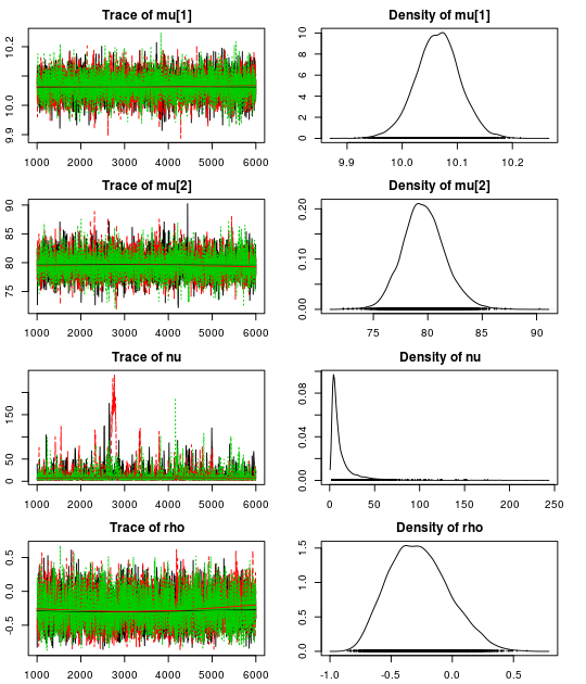
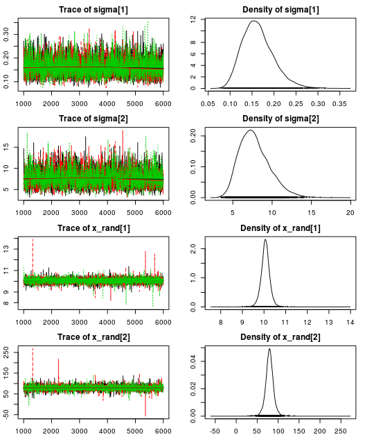
Here are the resulting trace plots and density plots…
par(mar = rep(2.2, 4))
plot(mcmc_samples)


.. and here is a summary of the parameter estimates:
summary(mcmc_samples)
##
## Iterations = 1001:6000
## Thinning interval = 1
## Number of chains = 3
## Sample size per chain = 5000
##
## 1. Empirical mean and standard deviation for each variable,
##    plus standard error of the mean:
##
##             Mean      SD Naive SE Time-series SE
## mu[1]     10.065  0.0403 0.000329       0.000510
## mu[2]     79.641  1.9707 0.016091       0.030294
## nu        13.703 19.9326 0.162749       1.426841
## rho       -0.270  0.2441 0.001993       0.003985
## sigma[1]   0.163  0.0359 0.000293       0.000665
## sigma[2]   7.786  1.9440 0.015872       0.040905
## x_rand[1] 10.065  0.2105 0.001719       0.001732
## x_rand[2] 79.523 10.0099 0.081731       0.085990
##
## 2. Quantiles for each variable:
##
##             2.5%    25%    50%    75%  97.5%
## mu[1]      9.984 10.039 10.065 10.091 10.144
## mu[2]     75.976 78.350 79.572 80.857 83.778
## nu         2.381  4.547  7.515 14.350 61.519
## rho       -0.691 -0.448 -0.285 -0.108  0.241
## sigma[1]   0.105  0.138  0.160  0.184  0.245
## sigma[2]   4.718  6.374  7.546  8.952 12.198
## x_rand[1]  9.654  9.948 10.066 10.183 10.471
## x_rand[2] 59.926 73.963 79.466 85.092 99.637
Using our robust model we get a correlation of -0.28 (95% CI:[-0.69, 0.24]) which is much closer to our initial -0.10 (95% CI: [-0.51, 0.35]). Looking at the estimate for the nu parameter we see that there is evidence for non-normality as the median nu is quite small: 7.5 (95% CI: [2.4, 61.5]).
What about data with no outliers?
So now we have two Bayesian versions of Pearson’s correlation test, one normal and one robust. Do we always have to make a choice which of these two models to use? No! I’ll go for the robust version any day, you see, it also estimates the heaviness of the tails of the bivariate t-distribution and if there is sufficient evidence in the data for normality the estimated t-distribution will be very close to a normal distribution. We can have the cake and eat it!
To show that this works I will now apply the robust model to the same data that I used in the last post which are 30 random draws from a bivariate normal distribution.
plot(x, xlim = c(-125, 125), ylim = c(-100, 150))

Running both the standard normal model and the robust t-distribution model on this data results in very similar estimates of the correlation:
quantile(rho_samples, c(0.025, 0.5, 0.975))
##    2.5%     50%   97.5%
## -0.8780 -0.7637 -0.5578
quantile(robust_rho_samples, c(0.025, 0.5, 0.975))
##    2.5%     50%   97.5%
## -0.8842 -0.7644 -0.5518
Looking at the estimate of nu we see that it is quite high which is what we would expect since the data is normal.
quantile(nu_samples, c(0.025, 0.5, 0.975))
##    2.5%     50%   97.5%
##   5.903  30.216 120.186