As the normal distribution is sort of the default choice when modeling continuous data (but not necessarily the best choice), the Poisson distribution is the default when modeling counts of events. Indeed, when all you know is the number of events during a certain period it is hard to think of any other distribution, whether you are modeling the
number of deaths in the Prussian army due to horse kicks or the
numer of goals scored in a football game. Like the t.test in R there is also a poisson.test that takes one or two samples of counts and spits out a p-value. But what if you have some counts, but don’t significantly feel like testing a null hypothesis? Stay tuned!
![]()
Bayesian First Aid is an attempt at implementing reasonable Bayesian alternatives to the classical hypothesis tests in R. For the rationale behind Bayesian First Aid see the original announcement. The development of Bayesian First Aid can be followed on GitHub. Bayesian First Aid is a work in progress and I’m grateful for any suggestion on how to improve it!
The Model
The original poisson.test function that comes with R is rather limited, and that makes it fairly simple to construct the Bayesian alternative. However, at first sight poisson.test may look more limited than it actually is. The one sample version just takes one count of events $x$ and the number of periods $T$ during which the number of events were counted. If your ice cream truck sold 14 ice creams during one day you would call the function like poisson.test(x = 14, T = 1). This seems limited, what if you have a number of counts, say you sell ice cream during a whole week, what to do then? The trick here is that you can add up the counts and the number of time periods and this will be perfectly fine. The code below will still give you an estimate for the underlying rate of ice cream sales per day:
ice_cream_sales = c(14, 16, 9, 18, 10, 6, 13)
poisson.test(x = sum(ice_cream_sales), T = length(ice_cream_sales))
Note that this only works if the counts are well modeled by the same Poisson distribution. If the ice cream sales are much higher on the weekends, adding up the counts might not be a good idea. poisson.test is also limited in that it can only handle two counts; you can compare the performance of your ice cream truck with just one competitor’s, no more. As the Bayesian alternative accepts the same input as poisson.test it inherits some of it’s limitations (but it can easily be extended, read on!). The model for the Bayesian First Aid alternative to the one sample possion.test is:
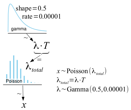
Here $x$ is again the count of events, $T$ is the number of periods, and $\lambda$ is the parameter of interest, the underlying rate at which the events occur. In the two sample case the one sample model is just separately fitted to each sample.
As $x$ is assumed to be Poisson distributed, all that is required to turn this into a fully Bayesian model is a prior on $\lambda$. In the the literature there are two common recommendations for an objective prior for the rate of a Poisson distribution. The first one is $p(\lambda) \propto 1 / \lambda$ which is the same as $p(log(\lambda)) \propto \text{const}$ and is proposed, for example, by Villegas (1977). While it can be argued that this prior is as non-informative as possible, it is problematic in that it will result in an improper posterior when the number of events is zero ($x = 0$). I feel that seeing zero events should tell the model something and, at least, not cause it to blow up. The second proposal is Jeffreys prior $p(\lambda) \propto 1 / \sqrt{\lambda}$, (as proposed by the great BUGS Book) which has a slight positive bias compared to the former prior but handles counts of zero just fine. The difference between these two priors is very small and will only matter when you have very few counts. Therefore the Bayesian First Aid alternative to poisson.test uses Jeffreys prior.
So if the model uses Jeffreys prior, what is the $\lambda \sim \text{Gamma}(0.5, 0.00001)$ doing in the model definition? Well, the computational framework underlying Bayesian First Aid is JAGS and in JAGS you build your model using probability distributions. The Jeffreys prior is not a proper probability distribution but it turns out that it can be reasonably well approximated by ${Gamma}(0.5, \epsilon)$ with $\epsilon \rightarrow 0$ (in the same way as $\lambda \propto 1 / \lambda$ can be approximated by ${Gamma}(\epsilon, \epsilon)$ with $\epsilon \rightarrow 0$).
The bayes.poisson.test Function
The bayes.poisson.test function accepts the same arguments as the original poisson.test function, you can give it one or two counts of events. If you just ran poisson.test(x=14, T=1), prepending bayes. runs the Bayesian First Aid alternative and prints out a summary of the model result (like bayes.poisson.test(x=14, T=1)). By saving the output, for example, like fit <- bayes.poisson.test(x=14, T=1) you can inspect it further using plot(fit), summary(fit) and diagnostics(fit).
To demonstrate the use of bayes.poisson.test I will use data from Boice and Monson (1977) on the number of women diagnosed with breast cancer in one group of 1,047 tuberculosis patients that had received on average 102 X-ray exams and one group of 717 tuberculosis patients whose treatment had not required a large number of X-ray exams. Here is the full data set:
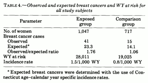
Here WY stand for woman-years (as if woman-years would be different from man-years, or person-years…). While the data is from a relatively old article we are going to replicate a more recent reanalysis of that data from the article Testing the Ratio of Two Poisson Rates by Gu et al. (2008). They tested the alternative hypothesis that the rate of breast cancer per person-year would be 1.5 times greater in the group that was X-rayed compared to the control group. They tested it like this:
no_cancer_cases <- c(41, 15)
# person-millennia rather than person-years to get the estimated rate
# on a more interpretable scale.
person_millennia <- c(28.011, 19.025)
poisson.test(no_cancer_cases, person_millennia, r = 1.5, alternative = "greater")
##
## 	Comparison of Poisson rates
##
## data:  no_cancer_cases time base: person_millennia
## count1 = 41, expected count1 = 41.61, p-value = 0.291
## alternative hypothesis: true rate ratio is greater than 1.5
## 95 percent confidence interval:
##  1.098   Inf
## sample estimates:
## rate ratio
##      1.856
and concluded that “There is not enough evidence that the incidence rate of breast cancer in the X-ray fluoroscopy group is 1.5 times to the incidence rate of breast cancer in control group”. It is oh-so-easy to interpret this as that there is no evidence that the incidence rate is more than 1.5 times higher, but this is wrong and the Bayesian First Aid alternative makes this clear:
library(BayesianFirstAid)
bayes.poisson.test(no_cancer_cases, person_millennia, r = 1.5, alternative = "greater")
## Warning: The argument 'alternative' is ignored by bayes.poisson.test
##
## 	Bayesian Fist Aid poisson test - two sample
##
## number of events: 41 and 15, time periods: 28.011 and 19.025
##
##   Estimates [95% credible interval]
## Group 1 rate: 1.5 [1.1, 1.9]
## Group 2 rate: 0.80 [0.43, 1.2]
## Rate ratio (Group 1 rate / Group 2 rate):
##               1.8 [1.1, 3.4]
##
## The event rate of group 1 is more than 1.5 times that of group 2 by a probability
## of 0.754 and less than 1.5 times that of group 2 by a probability of 0.246 .
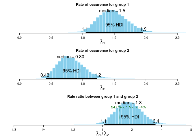
The warning here is nothing to worry about, there is no need to specify what alternative is tested and bayes.poisson.test just tells you that. So sure, the evidence is far from conclusive, but given the data and the model there is a 75% probability that the incidence rate is more than 1.5 times higher in the X-rayed group. That is, rather than just saying that there is not enough evidence we have quantified how much evidence there is, and the evidence actually slightly favors the alternative hypothesis. This is also easily seen in the default plot of bayes.poisson.test:
plot( bayes.poisson.test(no_cancer_cases, person_millennia, r = 1.5) )
Comparing More than Two Groups
Back to the ice cream truck, say that you sold 14 ice creams in one day and your competitors Karl and Anna sold 22 and 7 ice creams, respectively. How would you estimate and compare the underlying rates of sold ice creams of these three trucks when bayes.poisson.test only accepts counts from two groups? When you want to go off the beaten path the model.code function is your friend as it takes the result from Bayesian First Aid method and returns R and JAGS code that replicates the analysis you just ran. In this case start by running the model with two counts and then print out the model code:
fit <- bayes.poisson.test(x = c(14, 22), T = c(1, 1))
model.code(fit)
### Model code for the Bayesian First Aid two sample Poisson test ###
require(rjags)

# Setting up the data
x <- c(14, 22)
t <- c(1, 1)

# The model string written in the JAGS language
model_string <- "model {
  for(group_i in 1:2) {
    x[group_i] ~ dpois(lambda[group_i] * t[group_i])
    lambda[group_i] ~ dgamma(0.5, 0.00001)
    x_pred[group_i] ~ dpois(lambda[group_i] * t[group_i])
  }
  rate_diff <- lambda[1] - lambda[2]
  rate_ratio <- lambda[1] / lambda[2]
}"

# Running the model
model <- jags.model(textConnection(model_string), data = list(x = x, t = t), n.chains = 3)
samples <- coda.samples(model, c("lambda", "x_pred", "rate_diff", "rate_ratio"), n.iter=5000)

# Inspecting the posterior
plot(samples)
summary(samples)
Just copy-n-paste this code directly into an R script and make the following changes:
- Add the data for Karl’s ice cream truck:
x <- c(14, 22)→x <- c(14, 22, 7)t <- c(1, 1)→t <- c(1, 1, 1)
- Change the JAGS code so that you iterate over three groups instead of two:
for(group_i in 1:2) {→for(group_i in 1:3) {
And that’s it! Now we can run the model script and take a look at the estimated rates of ice cream sales for the three trucks.
plot(samples)
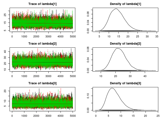
If you want to compare many groups you should perhaps consider using a hierarchical Poisson model. (Pro tip: John K. Kruschke’s Doing Bayesian Data Analysis has a great chapter on hierarchical Poisson models.)
References
Boice, J. D., & Monson, R. R. (1977). Breast cancer in women after repeated fluoroscopic examinations of the chest. Journal of the National Cancer Institute, 59(3), 823-832. link to article (unfortunatel behind paywall)
Gu, K., Ng, H. K. T., Tang, M. L., & Schucany, W. R. (2008). Testing the ratio of two poisson rates. Biometrical Journal, 50(2), 283-298. doi: 10.1002/bimj.200710403, pdf
Villegas, C. (1977). On the representation of ignorance. Journal of the American Statistical Association, 72(359), 651-654. doi: 10.2307/2286233
Lunn, D., Jackson, C., Best, N., Thomas, A., & Spiegelhalter, D. (2012). The BUGS book: a practical introduction to Bayesian analysis. CRC Press. pdf of chapter 5 on Prior distributions