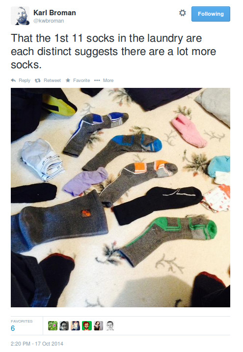
Big data is all the rage, but sometimes you don’t have big data. Sometimes you don’t even have average size data. Sometimes you only have eleven unique socks:
Karl Broman is here putting forward a very interesting problem. Interesting, not only because it involves socks, but because it involves what I would like to call Tiny Data™. The problem is this: Given the Tiny dataset of eleven unique socks, how many socks does Karl Broman have in his laundry in total?
If we had Big Data we might have been able to use some clever machine learning algorithm to solve this problem such as bootstrap aggregated neural networks. But we don’t have Big Data, we have Tiny Data. We can’t pull ourselves up by our bootstraps because we only have socks (eleven to be precise). Instead we will have to build a statistical model that includes a lot more problem specific information. Let’s do that!
Update: This post is now available as a 15 minute screencast: Tiny Data, Approximate Bayesian Computation and the Socks of Karl Broman: The Movie.
A Model of Picking out Socks from Your Laundry
We are going to start by building a generative model, a simulation of the I’m-picking-out-socks-from-my-laundry process. First we have a couple of parameters that I’m just for now are going to give arbitrary values:
n_socks <- 18 # The total number of socks in the laundry
n_picked <- 11 # The number of socks we are going to pick
In an ideal world all socks would come in pairs,
but we’re not living in an ideal world and some socks are odd (aka singletons). So out of the n_socks let’s say we have
n_pairs <- 7 # for a total of 7*2=14 paired socks.
n_odd <- 4
We are now going to create a vector of socks, represented as integers, where each pair/singleton is given a unique number.
socks <- rep( seq_len(n_pairs + n_odd), rep(c(2, 1), c(n_pairs, n_odd)) )
socks
## [1] 1 1 2 2 3 3 4 4 5 5 6 6 7 7 8 9 10 11
Finally we are going to simulate picking out n_picked socks (or at least n_socks if n_picked > n_socks) and counting the number of sock pairs and unique socks.
picked_socks <- sample(socks, size =  min(n_picked, n_socks))
sock_counts <- table(picked_socks)
sock_counts
## picked_socks
##  1  3  4  5  7  8  9 10 11
##  1  2  2  1  1  1  1  1  1
c(unique = sum(sock_counts == 1), pairs = sum(sock_counts == 2))
## unique  pairs
##      7      2
So for this particular run of the sock picking simulation we ended up with two pairs and seven unique socks. So far so good, but what about the initial problem? How to estimate the actual number of socks in Karl ’s laundry? Oh, but what you might not realize is that we are almost done! :)
Approximate Bayesian Computation for Socks Rocks
Approximate Bayesian Computation (ABC) is a super cool method for fitting models with the benefits of (1) being pretty intuitive and (2) only requiring the specification of a generative model, and with the disadvantages of (1) being extremely computationally inefficient if implemented naïvely and (2) requiring quite a bit of tweaking to work correctly when working with even quite small datasets. But we are not working with Quite Small Data, we are working with Tiny Data! Therefore we can afford a naïve and inefficient (but straight forward) implementation. Fiercely hand-waving, the simple ABC rejection algorithm goes like this:
- Construct a generative model that produces the same type of data as you are trying to model. Assume prior probability distributions over all the parameters that you want to estimate. Just as when doing standard Bayesian modelling these distributions represents the model’s information regarding the parameters before seeing any data.
- Sample tentative parameters values from the prior distributions, plug these into the generative model and simulate a dataset.
- Check if the simulated dataset matches the actual data you are trying to model. If yes, add the tentative parameter values to a list of retained probable parameter values, if no, throw them away.
- Repeat step 2 and 3 a large number of times building up the list of probable parameter values.
- Finally, the distribution of the probable parameter values represents the posterior information regarding the parameters. Intuitively, the more likely it is that a set of parameters generated data identical to the observed, the more likely it is that that combination of parameters ended up being retained.
For a less brief introduction to ABC see the tutorial on Darren Wilkinson’s blog. The paper by Rubin (1984) is also a good read, even if it doesn’t explicitly mention ABC.
Prior Sock Distributions
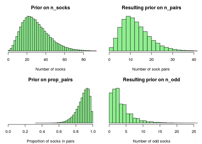
So what’s left until we can estimate the number of socks in Karl Broman’s laundry? Well, we have a reasonable generative model, however, we haven’t specified any prior distributions over the parameters we are interested in: n_socks, n_pairs and n_odd. Here we can’t afford to use non-informative priors, that’s a luxury reserved for the Big Data crowd, we need to use all the information we have. Also, the trade-off isn’t so much about how informative/biased we should be but rather about how much time/resources we can spend on developing reasonable priors. The following is what I whipped up in half an hour and which could surely be improved upon:
What can be said about n_socks, the number of socks in Karl Broman’s laundry, before seeing any data? Well, we know that n_socks must be positive (no anti-socks) and discrete (socks are not continuous). A reasonable choice would perhaps be to use a Poisson distribution as a prior, however the Poisson is problematic in that both its mean and its variance is set by the same parameter. Instead we could use the more flexible cousin to the Poisson, the negative binomial. In R the rnbinom function is parameterized with the mean mu and size. While size is not the variance, there is a direct correspondence between size and the variance s^2:
size = -mu^2 / (mu - s^2)
If you are a family of 3-4 persons and you change socks around 5 times a week then a guesstimate would be that you have something like 15 pairs of socks in the laundry. It is reasonable that you at least have some socks in your laundry, but it is also possible that you have much more than 15 * 2 = 30 socks. So as a prior for n_socks I’m going to use a negative binomial with mean prior_mu = 30 and standard deviation prior_sd = 15.
prior_mu <- 30
prior_sd <- 15
prior_size_param <- -prior_mu^2 / (prior_mu - prior_sd^2)
n_socks <- rnbinom(1, mu = prior_mu, size = prior_size_param)
Instead of putting a prior distribution directly over n_pairs and n_odd I’m going to put it over the proportion of socks that come in pairs prop_pairs. I know some people keep all their socks neatly paired, but only 3/4 of my socks are in a happy relationship. So on prop_pairs I’m going to put a Beta prior distribution that puts most of the probability over the range 0.75 to 1.0. Since socks are discrete entities we’ll also have to do some rounding to then go from prop_pairs to n_pairs and n_odd.
  prop_pairs <- rbeta(1, shape1 = 15, shape2 = 2)
  n_pairs <- round(floor(n_socks / 2) * prop_pairs)
  n_odd <- n_socks - n_pairs * 2

Bringing it All Together
Now we have a generative model, with reasonable priors, and what’s left is to use the ABC rejection algorithm to generate a posterior distribution of the number of socks in Karl Broman’s laundry. The following code bring all the earlier steps together and generates 100,000 samples from the generative model which are saved, together with the corresponding parameter values, in sock_sim:
n_picked <- 11 # The number of socks to pick out of the laundry

sock_sim <- replicate(100000, {
  # Generating a sample of the parameters from the priors
  prior_mu <- 30
  prior_sd <- 15
  prior_size <- -prior_mu^2 / (prior_mu - prior_sd^2)
  n_socks <- rnbinom(1, mu = prior_mu, size = prior_size)
  prop_pairs <- rbeta(1, shape1 = 15, shape2 = 2)
  n_pairs <- round(floor(n_socks / 2) * prop_pairs)
  n_odd <- n_socks - n_pairs * 2

  # Simulating picking out n_picked socks
  socks <- rep(seq_len(n_pairs + n_odd), rep(c(2, 1), c(n_pairs, n_odd)))
  picked_socks <- sample(socks, size =  min(n_picked, n_socks))
  sock_counts <- table(picked_socks)

  # Returning the parameters and counts of the number of matched
  # and unique socks among those that were picked out.
  c(unique = sum(sock_counts == 1), pairs = sum(sock_counts == 2),
    n_socks = n_socks, n_pairs = n_pairs, n_odd = n_odd, prop_pairs = prop_pairs)
})

# just translating sock_sim to get one variable per column
sock_sim <- t(sock_sim)
head(sock_sim)
##      unique pairs n_socks n_pairs n_odd prop_pairs
## [1,]      7     2      32      15     2     0.9665
## [2,]      7     2      21       9     3     0.9314
## [3,]      3     4      20       8     4     0.8426
## [4,]     11     0      47      23     1     0.9812
## [5,]      9     1      36      15     6     0.8283
## [6,]      7     2      16       5     6     0.6434
We have used quite a lot of prior knowledge, but so far we have not used the actual data. In order to turn our simulated samples sock_sim into posterior samples, informed by the data, we need to throw away those simulations that resulted in simulated data that doesn’t match the actual data. The data we have is that out of eleven picked socks, eleven were unique and zero were matched, so let’s remove all simulated samples which does not match this.
post_samples <- sock_sim[sock_sim[, "unique"] == 11 &
                         sock_sim[, "pairs" ] == 0 , ]
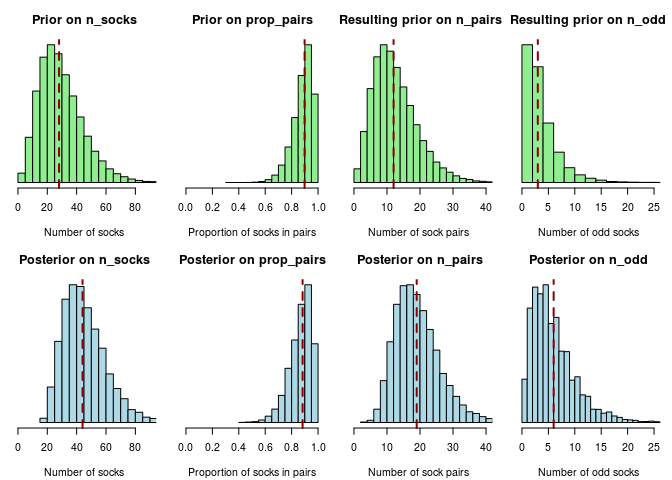
And we are done! Given the model and the data, the 11,506 remaining samples in post_samples now represent the information we have about the number of socks in Karl Broman’s laundry. What remains is just to explore what post_samples says about the number of socks. The following plot shows the prior sock distributions in green, and the posterior sock distributions (post_samples) in blue:

Here the vertical red lines show the median posterior, a “best guess” for the respective parameter. There is a lot of uncertainty in the estimates but our best guess (the median posterior) would be that there in Karl Broman’s laundry are 19 pairs of socks and 6 odds socks for a total of 19 × 2 + 6 = 44 socks.
How well did we do? Fortunately Karl Broman later tweeted the actual number of pairs and odd socks:
Which totals 21 × 2 + 3 = 45 socks. We were only off by one sock! Our estimate of the number of odd socks was a little bit high (Karl Broman is obviously much better at organizing his socks than me) but otherwise we are actually amazingly spot on! All thanks to carefully selected priors, approximate Bayesian computation and Tiny Data.
For full disclosure I must mention that Karl made this tweet before I had finished the model, however, I tried hard not to be influenced by that when choosing the priors of the model.
Coda and Criticism
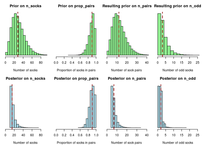
If you look at the plot of the priors and posteriors above you will notice that they are quite similar. “Did we even use the data?”, you might ask, “it didn’t really seem to make any difference anyway…”. Well, since we are working with Tiny Data it is only natural that the data does not make a huge difference. It does however make a difference. Without any data (also called No Data™) the median posterior number of socks would be 28, a much worse estimate than the Tiny Data estimate of 44. We could also see what would happen if we would fit the model to a different dataset. Say we got four pairs of socks and three unique socks out of the eleven picked socks. We would then calculate the posterior like this…
post_samples <- sock_sim[sock_sim[, "unique"] == 3 &
                         sock_sim[, "pairs" ] == 4 , ]
The posterior would look very different and our estimate of the number of total socks would be as low as 15:

So our Tiny Data does matter! There are, of course, other ways to criticize my model:
- Why did you use those priors? Well, those were the priors I came up with during the train trip I spent on developing this model. Especially the prior on the number of socks is a bit off since I believe it is more common to have an even number of socks in your laundry, something the prior does not consider.
- Why did you use approximate Bayesian computation instead of a likelihood based approach? Honestly, I haven’t really figured out (nor spent much time on) how to calculate the likelihood of the model. I would be very interested in a solution!
- Why didn’t you use another model? Why don’t you use another model? And show me! :) I think the problem proposed by Karl Broman is a pretty fun one, and the more models the merrier.
As a final note, don’t forget that you can follow Karl Broman on Twitter, he is a cool guy (even his tweets about laundry are thought provoking!) and if you aren’t already tired of clothes related analyses and Tiny Data you can follow me too :)
References
Rubin, D. B. (1984). Bayesianly justifiable and relevant frequency calculations for the applied statistician. The Annals of Statistics, 12(4), 1151-1172. full text

