In the last post I described flogs, a useful transform on proportions data introduced by John Tukey in his Exploratory Data Analysis. Flogging a proportion (such as, two out of three computers were Macs) consisted of two steps: first we “started” the proportion by adding 1/6 to each of the counts and then we “folded” it using what was basically a rescaled log odds transform. So for the proportion two out of three computers were Macs we would first add 1/6 to both the Mac and non-Mac counts resulting in the “started” proportion (2 + 1/6) / (2 + 1/6 + 1 + 1/6) = 0.65. Then we would take this proportion and transform it to the log odds scale.

The last log odds transform is fine, I’ll buy that, but what are we really doing when we are “starting” the proportions? And why start them by the “magic” number 1/6? Maybe John Tukey has the answer? From page 496 in Tukey’s EDA:

The desirability of treating “none seen below” as something other than zero is less clear, but also important. Here practice has varied, and a number of different usages exist, some with excuses for being and others without. The one we recommend does have an excuse but since this excuse (i) is indirect and (ii) involves more sophisticated considerations, we shall say no more about it. What we recommend is adding 1/6 to all […] counts, thus “starting” them.

Not particularly helpful… I don’t know what John Tukey’s original reason was (If you know, please tell me in the comments bellow!) but yesterday I figured out a reason that I’m happy with. Turns out that starting proportions by adding 1/6 to the counts is an approximation to the median of the posterior probability of the $\theta$ parameter of a Bernouli distribution when using Jeffrey’s prior on $\theta$. I’ll show you in a minute why this is the case but first I just want to point out that intuitively this is roughly what we would want to get when “starting” proportions.

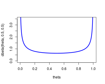
The reason for starting proportions in the first place was to gracefully handle cases such as 1/1 and 0/1 where the “raw” proportions would result in the edge proportions 100 % and 0 %. But surely we don’t believe that a person is a 100 % Apple fanboy just after getting to know that that person has one Mac computer out of in total one computer. That person is probably more likely to purchase a new Mac rather that a new PC but to estimate this probability as 100 % just after seeing one data point seems a bit rash. This kind of thinking is easily accommodated in a Bayesian framework by using a prior distribution on the proportion/probability parameter $\theta$ of the Bernoulli distribution that puts some prior probability on all possible proportions. One such prior is Jeffrey’s prior which is $\theta \sim Beta(0.5,0.5)$ and looks like this:

theta <- seq(0, 1, length.out = 1000)
plot(theta, dbeta(theta, 0.5, 0.5), type = "l", ylim = c(0, 3.5), col = "blue", 
    lwd = 3)

So instead of calculating the raw proportions we could estimate them using the following model:

$$x_i \sim \text{Bernouli}(\theta)$$

$$\theta \sim \text{Beta}(0.5,0.5)$$

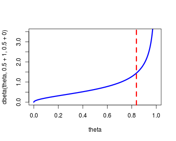
Here $x_i$ is a vector of zeroes and ones coding for, e.g., non-Macs (0) and Macs (1). This is easy to estimate using the fact that the posterior distribution of $\theta$ is given by $\text{Beta}(0.5 + n_1, 0.5 + n_0)$ where $n_0$ and $n_1$ are the number of zeroes and ones respectively. Running with our example of the guy with the one single Mac the estimated posterior distribution of the proportion $\theta$ would be:

theta <- seq(0, 1, length.out = 1000)
plot(theta, dbeta(theta, 0.5 + 1, 0.5 + 0), type = "l", ylim = c(0, 3.5), col = "blue", 
    lwd = 3)
abline(v = median(rbeta(99999, 0.5 + 1, 0.5 + 0)), col = "red", lty = 2, lwd = 3)

Now in order to get a single, point estimate out of this posterior distribution we have to summarize it in some way. One way is by taking the median as our “best guess” of the underlying value of $\theta$. The median of the distribution above is marked by the red, dashed line. It turns out that there is no easy, closed form expression for the median of a Beta distribution, however, the median can be approximated (according to Kerman , 2011) by

$$ \approx \frac{ \alpha - \tfrac{1}{3} }{ \alpha + \beta - \tfrac{2}{3} } $$

where $\alpha$ and $\beta$ are the values of the first and second parameters to the Beta distribution. In our case, with Jeffrey’s prior adding 0.5 to both parameters, we have:

$$\alpha = 0.5 + n_1$$

$$\beta = 0.5 + n_0$$

Substituting this into the expression above we get:

$$ \approx \frac{ 0.5 + n_1 - \tfrac{1}{3} }{ 0.5 + n_1 + 0.5 + n_0 - \tfrac{2}{3} } $$

which reduces to

$$ \approx \frac{n_1 + \tfrac{1}{6} }{n_1 + n_0 + \tfrac{1}{3} } $$

this is exactly the same expression as Tukey used to “start” proportions! Thus, the way Tukey calculate proportions is justifiable as the point estimate of a Bayesian estimation procedure.

Knowing this, it is possible to play around with the flog function I presented in the last post:

flog <- function(successes, failures, total_count = successes + failures) {
    p <- (successes + 1/6)/(total_count + 1/3)
    (1/2 * log(p) - 1/2 * log(1 - p))
}

Instead of using Jeffrey’s prior we might want to use a flat prior on $\theta$, as we believe that, initially, all values of $\theta$ are equally likely. A flat prior is given by the $\text{Beta}(1,1)$ distribution:

theta <- seq(0, 1, length.out = 1000)
plot(theta, dbeta(theta, 1, 1), type = "l", ylim = c(0, 2), col = "blue", lwd = 3)

Instead of using the median of the resulting posterior to produce a point value we might prefer taking the mean instead. The mean of a Beta distribution is just $\alpha / (\alpha + \beta)$. The flog function can easily be changed to accommodate these two changes as follows:

flog <- function(successes, failures, total_count = successes + failures) {
    p <- (successes + 1)/(total_count + 2)
    (1/2 * log(p) - 1/2 * log(1 - p))
}

So all of this is great, but I still wonder what Tukey’s original justification was for “starting” proportions in the way he did…

References

Kerman, J. (2011). A closed-form approximation for the median of the beta distribution. arXiv preprint arXiv:1111.0433. https://arxiv.org/abs/1111.0433