Student’s t-test is a staple of statistical analysis. A quick search on Google Scholar for “t-test” results in 170,000 hits in 2013 alone. In comparison, “Bayesian” gives 130,000 hits while “box plot” results in only 12,500 hits. To be honest, if I had to choose I would most of the time prefer a notched boxplot to a t-test. The t-test comes in many flavors: one sample, two-sample, paired samples and Welch’s. We’ll start with the two most simple; here follows the Bayesian First Aid alternatives to the one sample t-test and the paired samples t-test.

Bayesian First Aid is an attempt at implementing reasonable Bayesian alternatives to the classical hypothesis tests in R. For the rationale behind Bayesian First Aid see the original announcement and the description of the alternative to the binomial test. The development of Bayesian First Aid can be followed on GitHub. Bayesian First Aid is a work in progress and I’m grateful for any suggestion on how to improve it!
The Model
A straight forward alternative to the t-test would be to assume normality, add some non-informative priors to the mix and be done with it. However, one of great things with Bayesian data analysis is that it is easy to not assume normality. One alternative to the normal distribution, that still will fit normally distributed data well but that is more robust against outliers, is the t distribution. Hang on, you say, isn’t the t-test already using the t-distribution?. Right, the t-test uses the t-distribution as the distribution of the sample mean divided by the sample SD, here the trick is to assume it as the distribution of the data.
Instead of reinventing the wheel I’ll here piggyback on the work of John K. Kruschke who has developed a Bayesian estimation alternative to the t-test called Bayesian Estimation Supersedes the T-test, or BEST for short. The rationale and the assumptions behind BEST are well explained in a paper published 2013 in the Journal of Experimental Psychology (the paper is also a very pedagogical introduction to Bayesian estimation in general). That paper and more information regarding BEST is available on John Kruschkes web page. He has also made a nice video based on the paper (mostly focused on the two sample version though):
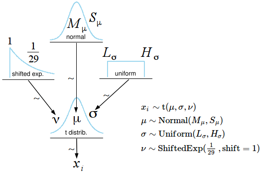
All information regarding BEST is given in the paper and the video, here is just a short rundown of the model for the one sample BEST: BEST assumes the data ($x$) is distributed as a t distribution which is more robust than a normal distribution due to its wider tails. Except for the mean ($\mu$) and the scale ($\sigma$) the t has one additional parameter, the degree-of-freedoms ($\nu$), where the lower $\nu$ is the wider the tails become. When $\nu$ gets larger the t distribution approaches the normal distribution. While it would be possible to fix $\nu$ to a single value BEST instead estimates $\nu$ allowing the t-distribution to become more or less normal depending on the data. Here is the full model for the one sample BEST:

The prior on $\nu$ is an exponential distribution with mean 29 shifted 1 to the right keeping $\nu$ away from zero. From the JEP 2013 paper: “This prior was selected because it balances nearly normal distributions ($\nu$ > 30) with heavy tailed distributions ($\nu$ < 30)”. The priors on $\mu$ and $\sigma$ are decided by the hyper parameters $M_\mu$, $S_\mu$, $L_\sigma$ and $H_\sigma$. By taking a peek at the data these parameters are set so that the resulting priors are extremely wide. While having a look at the data pre-analysis is generally not considered kosher, in practice this gives the same results as putting $\mathrm{Uniform}(-\infty,\infty)$ distributions on $\mu$ and $\sigma$.
The Model for Paired Samples
Here I use the simple solution. Instead of modeling the distribution of both groups and the paired differences the Bayesian First Aid alternative uses the same trick as the original paired samples t-test: Take the difference between each paired sample and model just the paired differences using the one sample procedure. Thus the alternative to the paired samples t-test is the same as the one sample alternative, the only difference is in how the data is prepared and the how the result is presented.
The bayes.t.test Function
The t.test function is used to run all four versions of the t-test. Here I’ll just show the one sample and paired samples alternatives. The bayes.t.test runs the Bayesian First Aid alternative to the t-test and has a function signature that is compatible with t.test function. That is, if you just ran a t-test, say t.test(x, conf.int=0.8, mu=1), just prepend bayes. and it should work out of the box.
The example data I’ll use to show off bayes.t.test is from the 2002 Nature article The Value of Bees to the Coffee Harvest (
doi:10.1038/417708a,
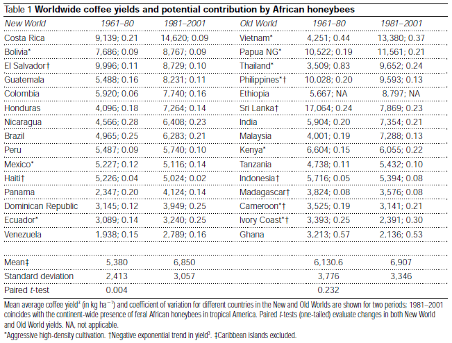
pdf). In this article David W. Roubik argues that bees are important to the coffee harvest despite that the “self-pollinating African shrub Coffea arabica, a pillar of tropical agriculture, was considered to gain nothing from insect pollinators”. Supporting the argument is a data set of the mean average coffee yield (in kg / 10,000 m) for new world countries in 1961-1980, before the establishment of African honeybees, and in 1981-2001, when African honeybees had been more or less been naturalized. This data shows an increased yield after the introduction of bees and when analyzed using a paired t-test results in p = 0.04. This is compared with the increase in yield in old world countries, where the bees been busy buzzing all along, were a paired t-test gives p = 0.232 interpreted as “no change”. The full dataset is given in the table below and in this csv file (to match the analysis in the paper the csv does not include the Caribbean islands)
There are a couple of reasons for why it is not proper to use a t-test to analyze this data set. A t-test does not consider the geographical location of the countries nor is it clear what “population” the sample of countries is drawn from. I also feel tempted to mutter the old cliché “correlation does not imply causation”, surely there must have been many things except for the introduction of bees that changed in Bolivia between 1961 and 2001. Being aware of these objections I’m going to use it to nevertheless show off the paired bayes.t.test.
Let’s first run the original analysis from the paper:
d <- read.csv("roubik_2002_coffe_yield.csv")
new_yield_80 <- d$yield_61_to_80[d$world == "new"]
new_yield_01 <- d$yield_81_to_01[d$world == "new"]
t.test(new_yield_01, new_yield_80, paired = TRUE, alternative = "greater")
##
## 	Paired t-test
##
## data:  new_yield_01 and new_yield_80
## t = 3.116, df = 12, p-value = 0.004464
## alternative hypothesis: true difference in means is greater than 0
## 95 percent confidence interval:
##  629 Inf
## sample estimates:
## mean of the differences
##                    1470
In the paper they used one tailed t-test hence the unhelpfully wide confidence interval. Now the Bayesian First Aid alternative:
library(BayesianFirstAid)
bayes.t.test(new_yield_01, new_yield_80, paired = TRUE, alternative = "less")
## Warning: The argument 'alternative' is ignored by bayes.binom.test
##
## 	Bayesian estimation supersedes the t test (BEST) - paired samples
##
## data: new_yield_01 and new_yield_80, n = 13
##
##   Estimates [95% credible interval]
## mean paired difference: 1422 [381, 2478]
## sd of the paired differences: 1755 [925, 2738]
##
## The mean difference is more than 0 by a probability of 0.994
## and less than 0 by a probability of 0.006
So here we get estimates for the mean and SD with credible intervals on the side. We also get to know that the probability that the mean increase is more than zero is 99.4%. We could also take a look at the data from the old world:
old_yield_80 <- d$yield_61_to_80[d$world == "old"]
old_yield_01 <- d$yield_81_to_01[d$world == "old"]
bayes.t.test(old_yield_01, old_yield_80, paired = TRUE)
##
## 	Bayesian estimation supersedes the t test (BEST) - paired samples
##
## data: old_yield_01 and old_yield_80, n = 15
##
##   Estimates [95% credible interval]
## mean paired difference: 716 [-1223, 2850]
## sd of the paired differences: 3551 [1104, 5761]
##
## The mean difference is more than 0 by a probability of 0.766
## and less than 0 by a probability of 0.234
So the trend here is also increasing yields, though the parameter estimate is much less precise and the 95% CI includes zero. Also notable is the much larger SD compare to the new world countries.
Generic Functions
Every Bayesian First Aid test have corresponding plot, summary, diagnostics and model.code functions. Here follows examples of these using the new world data.
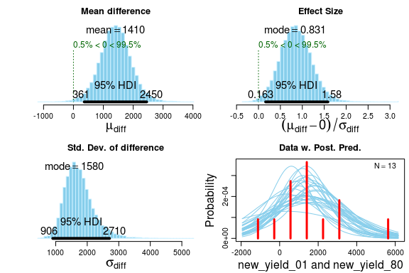
Using plot we get to look at the posterior distributions directly. We also get a posterior predictive check in the form of a histogram with a smattering of t-distributions drawn from the posterior. If there is a large discrepancy between the model fit and the data then we need to think twice before proceeding. As it is now I would say the post. pred. check looks OK.
fit <- bayes.t.test(new_yield_01, new_yield_80, paired = TRUE)
plot(fit)

summary gives us a detailed summary of the posterior. Note that the number of decimals places in this summary is a bit excessive, due to the posterior being approximated using MCMC the numbers will jump around slightly between runs. If this worries you increase the number of MCMC iterations by using the argument n.iter when calling bayes.t.test.
summary(fit)
##   Data
## new_yield_01, n = 13
## new_yield_80, n = 13
##
##   Model parameters and generated quantities
## mu_diff: the mean pairwise difference between new_yield_01 and new_yield_80
## sigma_diff: the standard deviation of the pairwise difference
## nu: the degrees-of-freedom for the t distribution fitted to the pairwise difference
## eff_size: the effect size calculated as (mu_diff - 0) / sigma_diff
## diff_pred: predicted distribution for a new datapoint generated
##   as the pairwise difference between new_yield_01 and new_yield_80
##
##   Measures
##                mean       sd     HDIlo    HDIup %<comp %>comp
## mu_diff    1408.417  525.511   360.853 2451.763  0.005  0.995
## sigma_diff 1747.749  470.010   906.023 2708.192  0.000  1.000
## nu           29.084   28.125     1.001   84.001  0.000  1.000
## eff_size      0.859    0.363     0.163    1.585  0.005  0.995
## diff_pred  1418.054 4250.459 -2762.415 5458.705  0.221  0.779
##
## 'HDIlo' and 'HDIup' are the limits of a 95% HDI credible interval.
## '%<comp' and '%>comp' are the probabilities of the respective parameter being
## smaller or larger than 0.
##
##   Quantiles
##                q2.5%     q25%   median     q75%   q97.5%
## mu_diff      366.882 1072.550 1404.144 1737.091 2458.905
## sigma_diff  1000.814 1428.718 1688.636 1991.766 2857.139
## nu             2.325    9.417   20.370   39.545  103.615
## eff_size       0.182    0.613    0.846    1.087    1.608
## diff_pred  -2724.139  180.476 1386.223 2600.898 5520.726
diagnostics prints and plots MCMC diagnostics (similar to the example in
bayes.binom.test). Finally model.code prints out R and JAGS code that replicates the analysis and that can be directly copy-n-pasted into an R script and modified from there. Here goes:
model.code(fit)
## Model code for Bayesian estimation supersedes the t test - paired samples ##
require(rjags)

# Setting up the data
x <- new_yield_01
y <- new_yield_80
pair_diff <- x - y
comp_mu <-  0

# The model string written in the JAGS language
model_string <- "model {
  for(i in 1:length(pair_diff)) {
    pair_diff[i] ~ dt( mu_diff , tau_diff , nu )
  }
  diff_pred ~ dt( mu_diff , tau_diff , nu )
  eff_size <- (mu_diff - comp_mu) / sigma_diff

  mu_diff ~ dnorm( mean_mu , precision_mu )
  tau_diff <- 1/pow( sigma_diff , 2 )
  sigma_diff ~ dunif( sigmaLow , sigmaHigh )
  # A trick to get an exponentially distributed prior on nu that starts at 1.
  nu <- nuMinusOne + 1
  nuMinusOne ~ dexp(1/29)
}"

# Setting parameters for the priors that in practice will result
# in flat priors on mu and sigma.
mean_mu = mean(pair_diff, trim=0.2)
precision_mu = 1 / (mad(pair_diff)^2 * 1000000)
sigmaLow = mad(pair_diff) / 1000
sigmaHigh = mad(pair_diff) * 1000

# Initializing parameters to sensible starting values helps the convergence
# of the MCMC sampling. Here using robust estimates of the mean (trimmed)
# and standard deviation (MAD).
inits_list <- list(
  mu_diff = mean(pair_diff, trim=0.2),
  sigma_diff = mad(pair_diff),
  nuMinusOne = 4)

data_list <- list(
  pair_diff = pair_diff,
  comp_mu = comp_mu,
  mean_mu = mean_mu,
  precision_mu = precision_mu,
  sigmaLow = sigmaLow,
  sigmaHigh = sigmaHigh)

# The parameters to monitor.
params <- c("mu_diff", "sigma_diff", "nu", "eff_size", "diff_pred")

# Running the model
model <- jags.model(textConnection(model_string), data = data_list,
                    inits = inits_list, n.chains = 3, n.adapt=1000)
update(model, 500) # Burning some samples to the MCMC gods....
samples <- coda.samples(model, params, n.iter=10000)

# Inspecting the posterior
plot(samples)
summary(samples)
If we believe, for example, that robustness is not such a big issue and would like to assume that the data is normally distributed rather than t distributed we just have to make some small adjustments to this script. In the model code we change dt into dnorm and remove the nu parameter resulting in this model:
model_string <- "model {
  for(i in 1:length(pair_diff)) {
    pair_diff[i] ~ dnorm( mu_diff , tau_diff)
  }
  diff_pred ~ dnorm( mu_diff , tau_diff)
  eff_size <- (mu_diff - comp_mu) / sigma_diff

  mu_diff ~ dnorm( mean_mu , precision_mu )
  tau_diff <- 1/pow( sigma_diff , 2 )
  sigma_diff ~ dunif( sigmaLow , sigmaHigh )
}"
We also has to remove the monitoring of the nu parameter.
# The parameters to monitor.
params <- c("mu_diff", "sigma_diff", "eff_size", "diff_pred")
And that’s all.
Some Comments
The bayes.t.test does not include all the functionality of BEST. Check out the
BEST package by John K. Kruschke and Mike Meredith for an R and JAGS implementation of BEST including power analysis and more. T-testable data was not that easy to get by and I browsed through a lot of papers before I found the examples with the bees. Wouldn’t it be nice if people actually published some data, well well… I did find two other fun examples of t-testable data if someone would be interested:
- Biomechanics: Rubber bands reduce the cost of carrying loads. The data is in the supplementary material.
- Chimpanzees Recruit the Best Collaborators. The data is in the paper.
