While reading up on quantile regression I found a really nice hack described in Bayesian Quantile Regression Methods (Lancaster & Jae Jun, 2010). It is called Jeffreys’ substitution posterior for the median, first described by Harold Jeffreys in his Theory of Probability, and is a non-parametric method for approximating the posterior of the median. What makes it cool is that it is really easy to understand and pretty simple to compute, while making no assumptions about the underlying distribution of the data. The method does not strictly produce a posterior distribution, but has been shown to produce a conservative approximation to a valid posterior (Lavine, 1995). In this post I will try to explain Jeffreys’ substitution posterior, give R-code that implements it and finally compare it with a classical non-parametric test, the Wilcoxon signed-rank test. But first a picture of Sir Harold Jeffreys:

Say we have a vector $x$ and we are interested in the median of the underlying distribution. The property of the median is that it sits smack in the middle of the distribution. We would expect that, on average, half of the datapoints of a vector generated from a distribution would fall to the left of the median (and so the other half would fall to the right). Now, given the vector $x$ of length $n$ and a candidate for the median $m$, let $n_l$ be the number of values that fall to the left of $m$ and $n_r$ be the number of values that fall to the right. If $m$ was the actual median the probability of getting the $n_l$ and $n_r$ that we actually got could be calculated as

$$ \text{The number of ways of selecting } n_l \text{ out of } n \text{ values in } x\over \text{The number of ways of placing the } n \text{ values in x into two categories } (n_l\text{ and } n_r) $$

Or using notation:

$${{n}\choose{n_l}} \big / 2^n$$

Here is an example:

Jeffreys proposed to use the probability ${{n}\choose{n_l}} \big / 2^n$ as a substitution for the likelihood, $p(x \mid m)$, and then calculate $p(m \mid x) \propto p(x \mid m) \cdot p(m)$.

By doing this we get something posterior-like we can do the usual stuff with, calculate credible intervals, calculate the probability that the median is smaller than this and that, etc. Before doing this we will just rewrite the substitution likelihood $p(x \mid m)$ to make it easier to work with. We can rewrite the $n_l$-combinations statement as

$${{n}\choose{n_l}} = {n! \over n_l!n_r!}$$

resulting in

$${{{n}\choose{n_l}} \big / 2^n} = {{{n! \over n_l!n_r!2^n}} }$$

If we change the candidate for the median $m$ the only numbers that are going to change are $n_l!$ and $n_r!$, $n!$ and $2^n$ stays the same. So, if we are interested in an expression that is proportional to the likelihood we could just use

$$ p(x \mid m) \propto {1 \over n_l!n_r!}$$

If we assume a uniform prior over $m$ we get that

$$p(m \mid x) \propto p(x \mid m) \propto {1 \over n_l!n_r!}$$

Great! Now we have a method to go from a vector of data, $x$, to a posterior probability for the median, $p(m \mid x)$.

Doing it in R

Using Jeffreys’ substitution posterior in R is pretty simple, but we have to be cautious not to run into numerical trouble. Directly calculating $1 / (n_l!n_r!)$ will only work for small datasets, already factorial(180) results in values so large that you’ll get an error in R. To overcome this problem we’ll do all the calculations on the log-scale as far as possible, using lfactorial instead. We’ll also use the fact that all candidate $m$ between two datapoints have the same likelihood, and so it suffices to calculate the likelihood once for each interval between two datapoints. First, here is the code for plotting the posterior:

# Generating some test data 
x <- rnorm(20, mean=0, sd=1)

x <- sort(x)
n <- length(x)
# Now calculating the "likelihood" for the median being
# in each of the intervals between the xs. Easily done with the following:
# 1 / (factorial(1:(n - 1)) * factorial((n - 1):1))
# but on the log-scale to avoid numerical problems
loglike <- 1 - ( lfactorial(1:(n - 1)) + lfactorial((n - 1):1) )
# Going back to the likelihood scale, subtracting max(loglike) to avoid 
# floating-point underflow.
like <- exp(loglike - max(loglike))
# Plotting with type="s" which plots a step function.
plot(x, c(like, 0), type="s", xlim=c(-2, 2), ylab="Likelihood (sort of)", xlab="median")

Nice, we got a plot of the posterior which looks sort of like a skyscraper, but this is alright, the posterior is supposed to be a step function. Looking at the plot we can see that, most likely, the median is between -0.5 and 1.0 (which seems alright as we actually know that the true median is 0.0). However, the representation of the posterior that we currently have in R is not very useful if we would want to calculate credible intervals or the probability of the median being higher than, for example 0.0. A more useful format would be to have a vector of random samples drawn from the posterior. This is also pretty easy to do in R, but first we need a helper function:

# A more numerically stable way of calculating log( sum( exp( x ))) Source:
# https://r.789695.n4.nabble.com/logsumexp-function-in-R-td3310119.html
logsumexp <- function(x) {
    xmax <- which.max(x)
    log1p(sum(exp(x[-xmax] - x[xmax]))) + x[xmax]
}

Then we calculate the proportional likelihood of the median being in each interval, transforms this into a probability, and finally use these probabilities to sample from the posterior. I’m going to be slightly sloppy and disregard the posterior that lies outside the range of the data, if we have more than a dozen datapoints this sloppiness is negligible.

# like * diff(x), but on the log scale. Calculates the proportional 
# likelihood of the median being in each interval like:
# c( like[1] * (x[2] - x[1]), like[2] * (x[3] - x[2]), ... )
interval_loglike <- loglike + log(diff(x))
# Normalizing the likelihood to get to the probability scale
interval_prob <- exp(interval_loglike - logsumexp(interval_loglike))
# Sampling intervals proportional to their probability
n_samples <- 10000
samp_inter <- sample.int(n - 1, n_samples, replace=TRUE, prob = interval_prob)
# Then, within each sampled interval, draw a uniform sample.
s <- runif(n_samples, x[samp_inter], x[samp_inter + 1]) 

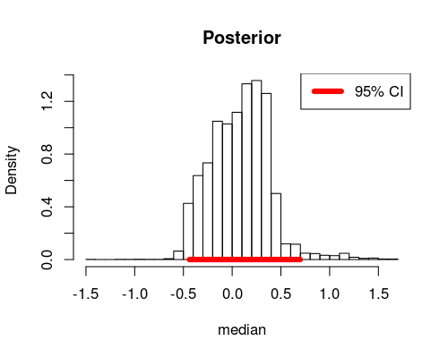
Now that we have a couple of samples in s we can do all the usual stuff such as calculating a 95% credible interval:

quantile(s, c(0.025, 0.975))

##    2.5%   97.5% 
## -0.4378  0.6978

or plotting the posterior as a histogram with a superimposed 95% CI:

hist(s, 30, freq = FALSE, main = "Posterior", xlab = "median")
lines(quantile(s, c(0.025, 0.975)), c(0, 0), col = "red", lwd = 6)
legend("topright", legend = "95% CI", col = "red", lwd = 6)

A Handy Function to Copy-n-Paste

Here is a handy function you should be able to copy-n-paste directly into R. It packages all the calculations done above into one function that plots the posterior, calculates a 95% CI and returns a vector of samples that can be further inspected. I haven’t tested this function extensively so use it at your own risk and please tell me if you find any bugs.

# A more numerically stable way of calculating log( sum( exp( x ))) Source:
# https://r.789695.n4.nabble.com/logsumexp-function-in-R-td3310119.html
logsumexp <- function(x) {
    xmax <- which.max(x)
    log1p(sum(exp(x[-xmax] - x[xmax]))) + x[xmax]
}

# Silently returns samples from Jeffreys’ substitution posterior given a
# vector of data (x). Also produces a histogram of the posterior and prints
# out a 95% quantile credible interval. Assumes a non-informative uniform
# [-Inf, Inf] prior over the median.
jeffreys_median <- function(x, n_samples = 10000, draw_plot = TRUE) {
    x <- sort(x)
    n <- length(x)
    loglike <- 1 - lfactorial(1:(n - 1)) - lfactorial((n - 1):1)
    interval_loglike <- loglike + log(diff(x))
    interval_prob <- exp(interval_loglike - logsumexp(interval_loglike))
    samp_inter <- sample.int(n - 1, n_samples, replace = TRUE, prob = interval_prob)
    s <- runif(n_samples, x[samp_inter], x[samp_inter + 1])
    cat("\n  Jeffreys’ Substitution Posterior for the median\n\n")
    cat("median\n  ", median(x), "\n")
    cat("95% CI\n  ", quantile(s, c(0.025, 0.975)), "\n")
    if (draw_plot) {
        hist(s, 30, freq = FALSE, main = "Posterior of the median", xlab = "median")
        lines(quantile(s, c(0.025, 0.975)), c(0, 0), col = "red", lwd = 5)
        legend("topright", legend = "95% CI", col = "red", lwd = 5)
    }
    invisible(s)
}

jeffreys_median vs wilcox.test

Finally, I thought I would compare Jeffreys’ substitution posterior with one of the most common classical non-parametric tests used, Wilcoxon signed-rank test. From the documentation for wilcox.test:

## Hollander & Wolfe (1973), 29f.  Hamilton depression scale factor
## measurements in 9 patients with mixed anxiety and depression, taken at the
## first (x) and second (y) visit after initiation of a therapy
## (administration of a tranquilizer).
x <- c(1.83, 0.5, 1.62, 2.48, 1.68, 1.88, 1.55, 3.06, 1.3)
y <- c(0.878, 0.647, 0.598, 2.05, 1.06, 1.29, 1.06, 3.14, 1.29)
wilcox.test(y - x, alternative = "less")

## 
##  Wilcoxon signed rank test
## 
## data:  y - x
## V = 5, p-value = 0.01953
## alternative hypothesis: true location is less than 0

So wilcox.test gives us a pretty small p-value, which could be taken to support that the distribution of y - x is not symmetric about 0.0, but not much more. Let’s rerun the analysis but using the R function we defined earlier.

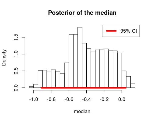
s <- jeffreys_median(y - x)

## 
##   Jeffreys’ Substitution Posterior for the median
## 
## median
##    -0.49 
## 95% CI
##    -0.9133 0.04514

Looking at the posterior we see that the most likely median difference is around -0.5, but the difference is also likely to be as negative as -1 and as positive as 0.1. Using the samples s we can calculate the probability that the median difference is less than 0:

mean(s < 0)

## [1] 0.9523

So, given the data and Jeffreys’ substitution posterior there is more than 95% probability that the median difference is less than 0. Compared with Wilcoxon signed-rank test I think Jeffreys’ substitution posterior is a good alternative when you are interested in the median but otherwise want to make as few assumptions as possible. However, I don’t want to generally recommend Jeffreys’ substitution posterior, as it doesn’t make strong assumptions almost any other model based on reasonable assumptions will be more powerful and will make better use of the data. Still, I think Jeffreys’ substitution posterior is a cool method with a clean, intuitive definition, and I just wonder: Why isn’t it better known?

References

Jeffreys, H. (1961). Theory of Probability. Clarendon Press: Oxford. Amazon link

Lancaster, T., & Jae Jun, S. (2010). Bayesian quantile regression methods. Journal of Applied Econometrics, 25(2), 287-307. pdf

Lavine, M. (1995). On an approximate likelihood for quantiles. Biometrika, 82(1), 220-222. link (unfortunately behind paywall)

{% endraw %}