Does pill A or pill B save the most lives? Which web design results in the most clicks? Which in vitro fertilization technique results in the largest number of happy babies? A lot of questions out there involves estimating the proportion or relative frequency of success of two or more groups (where success could be a saved life, a click on a link, or a happy baby) and there exists a little known R function that does just that, prop.test. Here I’ll present the Bayesian First Aid version of this procedure. A word of caution, the example data I’ll use is mostly from the
Journal of Human Reproduction and as such it might be slightly NSFW :)

Bayesian First Aid is an attempt at implementing reasonable Bayesian alternatives to the classical hypothesis tests in R. For the rationale behind Bayesian First Aid see the original announcement. The development of Bayesian First Aid can be followed on GitHub. Bayesian First Aid is a work in progress and I’m grateful for any suggestion on how to improve it!
The Model
This is a straight forward extension of
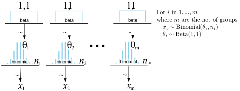
the Bayesian First Aid alternative to the binomial test which can be used to estimate the underlying relative frequency of success given a number of trials and, out of them, a number of successes. The model for bayes.prop.test is just more of the same thing, we’ll just estimate the relative frequencies of success for two or more groups instead. Below is the full model where $\theta_i$ is the relative frequency of success estimated given $x_i$ successes out of $n_i$ trials:
The bayes.prop.test Function
The bayes.prop.test function accepts the same arguments as the original prop.test function, you can give it two vectors one with counts of successes and one with counts of trials or you can supply the same data as a matrix with two columns. If you just ran prop.test(successes, trials), prepending bayes. (like bayes.prop.test(successes, trials)) runs the Bayesian First Aid alternative and prints out a summary of the model result. By saving the output, for example, like fit <- bayes.prop.test(successes, trials) you can inspect it further using plot(fit), summary(fit) and diagnostics(fit).
To demonstrate the use of bayes.prop.test I will use data from
the Kinsey Institute for Research in Sex, Gender and Reproduction as described in the article Genital asymmetry in men by
Bogaert (1997). The data consists of survey answers from 6544 “postpubertal males with no convictions for felonies or misdemeanours” where the respondents, among other things, were asked two questions:
- Are you right or left handed?
- If you were standing up and had an erection, if you looked down at the penis, would it be pointing straight ahead or pointed somewhat to the right or left?
I don’t know about you, but the first question I had was are right handed people more like to have it on the right, or perhaps the oposite? Here is the raw data given by Bogaert:
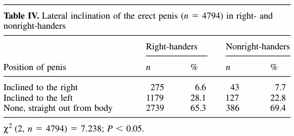
Seems like we have 4794 complete cases. Just looking at those with right or leftward disposition leaves us 1624 cases with 275 right leaners out of 1454 right-handers and 43 right leaners out of 170 non-right-handers. Bogaert uses a chi-square test to analyze this data but since we are interested in comparing proportions we’ll start with using prop.test instead:
# Below, the data from the right handers are on the right, logical right? :)
n_right_leaners <- c(43, 275)
n_respondents <- c(170, 1454)
prop.test(n_right_leaners, n_respondents)
##
## 	2-sample test for equality of proportions with continuity
## 	correction
##
## data:  n_right_leaners out of n_respondents
## X-squared = 3.541, df = 1, p-value = 0.05989
## alternative hypothesis: two.sided
## 95 percent confidence interval:
##  -0.007852  0.135468
## sample estimates:
## prop 1 prop 2
## 0.2529 0.1891
Not too bad, we get both a confidence interval on the difference between the groups and maximum likelihood estimates. Let’s compare this with the Bayesian First Aid version:
bayes.prop.test(n_right_leaners, n_respondents)
##
## 	Bayesian First Aid propotion test
##
## data: n_right_leaners out of n_respondents
## number of successes:    43,  275
## number of trials:      170, 1454
## Estimated relative frequency of success [95% credible interval]:
##   Group 1: 0.26 [0.19, 0.32]
##   Group 2: 0.19 [0.17, 0.21]
## Estimated group difference (Group 1 - Group 2):
##   0.07 [-0.0025, 0.13]
## The relative frequency of success is larger for Group 1 by a probability
## of 0.977 and larger for Group 2 by a probability of 0.023 .
Pretty similar estimates (and they should be) but now we also get estimates [and credible intervals] for both groups and the group difference. Looking at the estimates it seems like both left and right-handers tend to lean to the left much more often than to the right. We also get to know that the probability that left-handers lean more often to the right compared to right-handers is 97.7%. Interesting! Let’s look at this relation further by plotting the posterior distribution:
fit <- bayes.prop.test(n_right_leaners, n_respondents)
plot(fit)
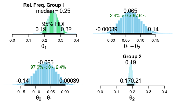
So, it is most likely that left-handers lean more to the right by around 6-7 percentage points (and Bogaert discusses some reasons why this might be the case). Still the posterior of the group difference is pretty wide (and the credible interval kisses the 0.0) and even though the analysis is leaning (he he) towards there being a difference it would be nice to have a few more data points to get a tighter estimate.
Using bayes.prop.test as a Replacement for chisq.test
I don’t like Pearson’s chi-squared test, it is used as a catch-all analysis for any tables of counts and what you get back is utterly uninformative: a p-value relating to the null hypothesis that the row variable is completely independent of the column variable (which is anyway known to be false a priori most of the time, see
here and
here for some discussion). If you have counts of successes for many groups and are interested in actually estimating group differences bayes.prop.test can also be used as a replacement for chisq.test. Let’s look at an example, again with data from the
Journal of Human Reproduction.
When doing in vitro fertilization the egg is fertilized by sperm outside the body and later, if successfully fertilized, reinserted into the uterus. The egg and the sperms are usually left together to co-incubate for more than an hour before the egg is separated from the sperm and left to incubate for itself. Bungum et al. (2006) was interested in comparing if an ultra-short co-incubation period of 30 s. would work as well as a more conventional co-incubation period of 90 m. Bungum et al. used a 30 s. co-incubation period on 389 eggs and a 90 min. period on another batch of 388 eggs and looked at a number of measures such as the number of fertilized eggs and the number of resulting embryos graded as high quality. Their analysis of the result is summarized in the table below:
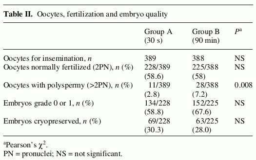
Unfortunately they use chi-square tests to analyze these counts and they don’t even report the full p-values, for all but one of the measures all we get to know is NS. Just looking at the raw data it seems like there is little difference between the proportions of fertilized eggs in the two groups, but there seems to be a difference in embryo quality with more embryos in the 90 min. group being of high quality (defined as grade 0 and 1). But the chi-square analysis says NS which is interpreted in the result section as: “the two groups were comparable”. Let’s analyze the data with bayes.prop.test:
no_good_grade <- c(134, 152)
no_embryos <- c(228, 225)
fit <- bayes.prop.test(no_good_grade, no_embryos)
plot(fit)
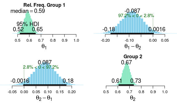
Looking at the posterior it seems like there is actually some evidence for that the 30 s. procedure results in fewer embryos of good quality as most of the posterior probability is centered around a difference of 6-12% percentage points. Sure, the credible interval kisses zero, but the evidence for a small difference, which was hinted at in the original article, is definitely not strong.
Using the concept of a region of practical equivalence (ROPE) we can calculate the probability that the difference between the two procedures is small. First we have to decide what would count as a small enough difference to be negligible. I have no strong intuition about what would be a small difference in this particular case, so I’m arbitrarily going to go with 5 percentage points, yielding a ROPE of [-5, 5] percentage points (for more about ROPEs see
Kruschke, 2011). To calculate the probability that the difference between the two groups is within the ROPE I’ll extract the MCMC samples generated when the model was fit using as.data.frame and then I’ll use them to calculate the probability “by hand”:
s <- as.data.frame(fit)
mean(abs((s$theta1 - s$theta2)) < 0.05)
## [1] 0.201
The probability that the relative frequency of high quality embryos is practically equivalent between the two procedures is only 20%, thus the probability that there is a substantial difference is 80%. There is definitely weak evidence for “no difference” here but we would need more data to be able state the magnitude of the difference with reasonable certainty.
Caveat: I know very little about in vitro fertilization and this is definitely not a critique of the study in any way. I don’t know what would be considered a region of practical equivalence in this case and I don’t know if embryo quality is considered an important outcome. However, I still believe that the analysis would have been more informative if they would have used something better than chi-square tests and p-values!
Comparing Many Groups
Like prop.test, bayes.prop.test can be used to compare more than two groups. Here is an example with a dataset from the prop.test help file on the number of smokers in four groups of patients with lung cancer.
smokers  <- c( 83, 90, 129, 70 )
patients <- c( 86, 93, 136, 82 )
fit <- bayes.prop.test(smokers, patients)
fit
##
## 	Bayesian First Aid propotion test
##
## data: smokers out of patients
## number of successes:   83,  90, 129,  70
## number of trials:      86,  93, 136,  82
## Estimated relative frequency of success [95% credible interval]:
##   Group 1: 0.96 [0.91, 0.99]
##   Group 2: 0.96 [0.92, 0.99]
##   Group 3: 0.94 [0.90, 0.98]
##   Group 4: 0.85 [0.77, 0.92]
## Estimated pairwise group differences (row - column) with 95 % cred. intervals:
##                         Group
##            2               3               4
##   1        0             0.01            0.11
##     [-0.063, 0.058] [-0.05, 0.068]   [0.023, 0.2]
##   2                      0.02            0.11
##                     [-0.042, 0.071]  [0.023, 0.2]
##   3                                       0.1
##                                      [0.013, 0.19]
plot(fit)
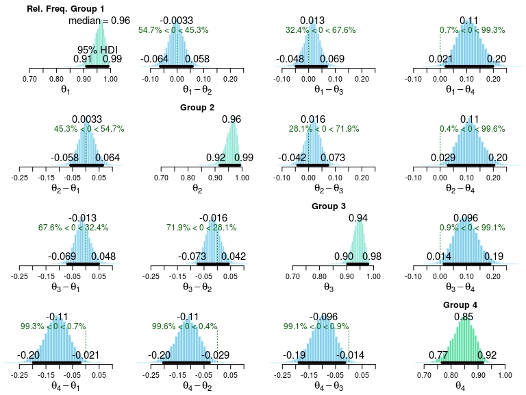
As is shown both in the print out and in the plot, group 4 seems to differ slightly from the rest. While bayes.prop.test can be used to compare more than four groups both the printouts and the plots start to get a bit overwhelming when there are too many groups. A remedy for this is to use the model.code function that prints out JAGS and R code that replicates the model you have fitted with bayes.prop.test and to customize this code further to make the plots and comparisons you are interested in.
model.code(fit)
### Model code for the Bayesian First Aid  ###
### alternative to the test of proportions ###
require(rjags)

# Setting up the data
x <- c(83, 90, 129, 70)
n <- c(86, 93, 136, 82)

# The model string written in the JAGS language
model_string <- "model {
  for(i in 1:length(x)) {
    x[i] ~ dbinom(theta[i], n[i])
    theta[i] ~ dbeta(1, 1)
    x_pred[i] ~ dbinom(theta[i], n[i])
  }
}"

# Running the model
model <- jags.model(textConnection(model_string), data = list(x = x, n = n),
                    n.chains = 3, n.adapt=1000)
samples <- coda.samples(model, c("theta", "x_pred"), n.iter=5000)

# Inspecting the posterior
plot(samples)
summary(samples)

# You can extract the mcmc samples as a matrix and compare the thetas
# of the groups. For example, the following shows the median and 95%
# credible interval for the difference between Group 1 and Group 2.
samp_mat <- as.matrix(samples)
quantile(samp_mat[, "theta[1]"] - samp_mat[, "theta[2]"], c(0.025, 0.5, 0.975))
Another reason to modify the code that is printed out by model.code is in order to change the assumptions of the model. The current model does not assume any dependency between the groups and if this is an unreasonable assumption you might want to modify the model code to include such a dependency. A nice example of how to extend the model to assume a hierarchical dependency between the relative frequencies of success of each group can be found on the
LingPipe blog. Hierarchical binomial models are also discussed in chapter 9 in Kruschke’s Doing Bayesian Data Analysis and in section 5.3 in Gelman et al.’s Bayesian Data Analysis.
References
Bogaert, A. F. (1997). Genital asymmetry in men. Human reproduction, 12(1), 68-72. doi: 10.1093/humrep/12.1.68 . pdf
Bungum, M., Bungum, L., & Humaidan, P. (2006). A prospective study, using sibling oocytes, examining the effect of 30 seconds versus 90 minutes gamete co-incubation in IVF. Human Reproduction, 21(2), 518-523. doi: 10.1093/humrep/dei350
Kruschke, J. K. (2011). Bayesian assessment of null values via parameter estimation and model comparison. Perspectives on Psychological Science, 6(3), 299-312. doi: 10.1177/1745691611406925 . pdf