Everybody loves speed comparisons! Is R faster than Python? Is dplyr faster than data.table? Is STAN faster than JAGS? It has been said that speed comparisons are utterly meaningless, and in general I agree, especially when you are comparing apples and oranges which is what I’m going to do here. I’m going to compare a couple of alternatives to lm(), that can be used to run linear regressions in R, but that are more general than lm(). One reason for doing this was to see how much performance you’d loose if you would use one of these tools to run a linear regression (even if you could have used lm()). But as speed comparisons are utterly meaningless, my main reason for blogging about this is just to highlight a couple of tools you can use when you grown out of lm(). The speed comparison was just to lure you in. Let’s run!

The Contenders

Below are the seven different methods that I’m going to compare by using each method to run the same linear regression. If you are just interested in the speed comparisons, just scroll to the bottom of the post. And if you are actually interested in running standard linear regressions as fast as possible in R, then Dirk Eddelbuettel has a nice post that covers just that.

lm()

This is the baseline, the “default” method for running linear regressions in R. If we have a data.frame d with the following layout:

head(d)

##         y      x1      x2
## 1 -64.579 -1.8088 -1.9685
## 2 -19.907 -1.3988 -0.2482
## 3  -4.971  0.8366 -0.5930
## 4  19.425  1.3621  0.4180
## 5  -1.124 -0.7355  0.4770
## 6 -12.123 -0.9050 -0.1259

Then this would run a linear regression with y as the outcome variable and x1 and x2 as the predictors:

lm(y ~ 1 + x1 + x2, data=d)

## 
## Call:
## lm(formula = y ~ 1 + x1 + x2, data = d)
## 
## Coefficients:
## (Intercept)           x1           x2  
##      -0.293       10.364       21.225

glm()

This is a generalization of lm() that allows you to assume a number of different distributions for the outcome variable, not just the normal distribution as you are stuck with when using lm(). However, if you don’t specify any distribution glm() will default to using a normal distribution and will produce output identical to lm():

glm(y ~ 1 + x1 + x2, data=d)

## 
## Call:  glm(formula = y ~ 1 + x1 + x2, data = d)
## 
## Coefficients:
## (Intercept)           x1           x2  
##      -0.293       10.364       21.225  
## 
## Degrees of Freedom: 29 Total (i.e. Null);  27 Residual
## Null Deviance:	    13200 
## Residual Deviance: 241 	AIC: 156

bayesglm()

Found in the arm package, this is a modification of glm that allows you to assume custom prior distributions over the coefficients (instead of the implicit flat priors of glm()). This can be super useful, for example, when you have to deal with perfect separation in logistic regression or when you want to include prior information in the analysis. While there is bayes in the function name, note that bayesglm() does not give you the whole posterior distribution, only point estimates. This is how to run a linear regression with flat priors, which should give similar results as when using lm():

library(arm)
bayesglm(y ~ 1 + x1 + x2, data = d, prior.scale=Inf, prior.df=Inf)

## 
## Call:  bayesglm(formula = y ~ 1 + x1 + x2, data = d, prior.scale = Inf, 
##     prior.df = Inf)
## 
## Coefficients:
## (Intercept)           x1           x2  
##      -0.293       10.364       21.225  
## 
## Degrees of Freedom: 29 Total (i.e. Null);  30 Residual
## Null Deviance:	    13200 
## Residual Deviance: 241 	AIC: 156

nls()

While lm() can only fit linear models, nls() can also be used to fit non-linear models by least squares. For example, you could fit a sine curve to a data set with the following call: nls(y ~ par1 + par2 * sin(par3 + par4 * x )). Notice here that the syntax is a little bit different from lm() as you have to write out both the variables and the parameters. Here is how to run the linear regression:

nls(y ~ intercept + x1 * beta1 + x2 * beta2, data = d)

## Nonlinear regression model
##   model: y ~ intercept + x1 * beta1 + x2 * beta2
##    data: d
## intercept     beta1     beta2 
##    -0.293    10.364    21.225 
##  residual sum-of-squares: 241
## 
## Number of iterations to convergence: 1 
## Achieved convergence tolerance: 3.05e-08

mle2()

In the bblme package we find mle2(), a function for general maximum likelihood estimation. While mle2() can be used to maximize a handcrafted likelihood function, it also has a formula interface which is simple to use, but powerful, and that plays nice with R’s built in distributions. Here is how to roll a linear regression:

library(bbmle)
inits <- list(log_sigma = rnorm(1), intercept = rnorm(1),
              beta1 = rnorm(1), beta2 = rnorm(1))
mle2(y ~ dnorm(mean = intercept + x1 * beta1 + x2 * beta2, sd = exp(log_sigma)),
     start = inits, data = d)

## 
## Call:
## mle2(minuslogl = y ~ dnorm(mean = intercept + x1 * beta1 + x2 * 
##     beta2, sd = exp(log_sigma)), start = inits, data = d)
## 
## Coefficients:
## log_sigma intercept     beta1     beta2 
##    1.0414   -0.2928   10.3641   21.2248 
## 
## Log-likelihood: -73.81

Note, that we need to explicitly initialize the parameters before the maximization and that we now also need a parameter for the standard deviation. For an even more versatile use of the formula interface for building statistical models, check out the very cool rethinking package by Richard McElreath.

optim()

Of course, if we want to be really versatile, we can craft our own log-likelihood function to maximized using optim(), also part of base R. This gives us all the options, but there are also more things that can go wrong: We might make mistakes in the model specification and if the search for the optimal parameters is not initialized well the model might not converge at all! A linear regression log-likelihood could look like this:

log_like_fn <- function(par, d) {
  sigma <- exp(par[1])
  intercept <- par[2]
  beta1 <- par[3]
  beta2 <- par[4]
  mu <- intercept + d$x1 * beta1 + d$x2 * beta2
  sum(dnorm(d$y, mu, sigma, log=TRUE))
}

inits <- rnorm(4)
optim(par = inits, fn = log_like_fn, control = list(fnscale = -1), d = d)

## $par
## [1]  1.0399 -0.2964 10.3637 21.2139
## 
## $value
## [1] -73.81
## 
## $counts
## function gradient 
##      431       NA 
## 
## $convergence
## [1] 0
## 
## $message
## NULL

As the convergence returned 0 it hopefully worked fine (a 1 indicates non-convergence). The control = list(fnscale = -1) argument is just there to make optim() do maximum likelihood estimation rather than minimum likelihood estimation (which must surely be the worst estimation method ever).

Stan’s optimizing()

Stan is a stand alone program that plays well with R, and that allows you to specify a model in Stan’s language which will compile down to very efficient C++ code. Stan was originally built for doing Hamiltonian Monte Carlo, but now also includes an optimizing() function that, like R’s optim(), allows you to do maximum likelihood estimation (or maximum a posteriori estimation, if you explicitly included priors in the model definition). Here we need to do a fair bit of work before we can fit a linear regression but what we gain is extreme flexibility in extending this model, would we need to. We have come a long way from lm…

library(rstan)

## Loading required package: inline
## 
## Attaching package: 'inline'
## 
## The following object is masked from 'package:Rcpp':
## 
##     registerPlugin
## 
## rstan (Version 2.6.0, packaged: 2015-02-06 21:02:34 UTC, GitRev: 198082f07a60)
## 
## Attaching package: 'rstan'
## 
## The following object is masked from 'package:arm':
## 
##     traceplot

model_string <- "
data {
  int n;
  vector[n] y;
  vector[n] x1;
  vector[n] x2;
}

parameters {
  real intercept;
  real beta1;
  real beta2;
  real<lower=0> sigma;
}

model {
  vector[n] mu;
  mu <- intercept + x1 * beta1 + x2 * beta2;
  y ~ normal(mu, sigma);
}
"

data_list <- list(n = nrow(d), y = d$y, x1 = d$x1, x2 = d$x2)
model <- stan_model(model_code = model_string)
fit <- optimizing(model, data_list)
fit

## $par
## intercept     beta1     beta2     sigma 
##   -0.2929   10.3642   21.2248    2.8331 
## 
## $value
## [1] -46.24

An Utterly Meaningless Speed Comparison

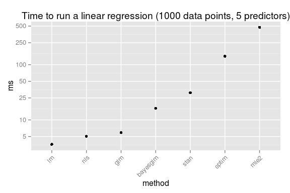
So, just for fun, here is the speed comparison, first for running a linear regression with 1000 data points and 5 predictors:

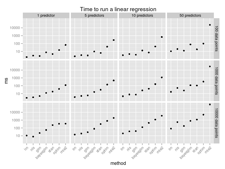
This should be taken with a huge heap of salt (which is not too good for your health!). While all these methods produce a result equivalent to a linear regression they do it in different ways, and not necessary in equally good ways, for example, my homemade optim routine is not converging correctly when trying to fit a model with too many predictors. As I have used the standard settings there is surely a multitude of ways in which any of these methods can be made faster. Anyway, here is what happens if we vary the number of predictors and the number of data points:

To make these speed comparisons I used the microbenchmark package, the full script replicating the plots above can be found here. This speed comparison was made on my laptop running R version 3.1.2, on 32 bit Ubuntu 12.04, with an average amount of RAM and a processor that is starting to get a bit tired.