The non-parametric bootstrap was my first love. I was lost in a muddy swamp of zs, ts and ps when I first saw her. Conceptually beautiful, simple to implement, easy to understand (I thought back then, at least). And when she whispered in my ear, “I make no assumptions regarding the underlying distribution”, I was in love. This love lasted roughly a year, but the more I learned about statistical modeling, especially the Bayesian kind, the more suspect I found the bootstrap. It is most often explained as a procedure, not a model, but what are you actually assuming when you “sample with replacement”? And what is the underlying model?

Still, the bootstrap produces something that looks very much like draws from a posterior and there are papers comparing the bootstrap to Bayesian models (for example, Alfaro et al., 2003). Some also wonder which alternative is more appropriate: Bayes or bootstrap? But these are not opposing alternatives, because the non-parametric bootstrap is a Bayesian model.

In this post I will show how the classical non-parametric bootstrap of Efron (1979) can be viewed as a Bayesian model. I will start by introducing the so-called Bayesian bootstrap and then I will show three ways the classical bootstrap can be considered a special case of the Bayesian bootstrap. So basically this post is just a rehash of Rubin’s The Bayesian Bootstrap from 1981. Some points before we start:

• Just because the bootstrap is a Bayesian model doesn’t mean it’s not also a frequentist model. It’s just different points of view.

• Just because it’s Bayesian doesn’t necessarily mean it’s any good. “We used a Bayesian model” is as much a quality assurance as “we used probability to calculate something”. However, writing out a statistical method as a Bayesian model can help you understand when that method could work well and how it can be made better (it sure helps me!).

• Just because the bootstrap is sometimes presented as making almost no assumptions, doesn’t mean it does. Both the classical non-parametric bootstrap and the Bayesian bootstrap make very strong assumptions which can be pretty sensible and/or weird depending on the situation.

Update: If you actually want to perform a Bayesian bootstrap you should check out my post Easy Bayesian Bootstrap in R.

The bootstrap as a Bayesian model, version one

Let’s start with describing the Bayesian bootstrap of Rubin (1981), which the classical bootstrap can be seen as a special case of. Let $d = (d_1, \ldots, d_K)$ be a vector of all the possible values (categorical or numerical) that the data $x = (x_1, \ldots, x_N)$ could possibly take. It might sound strange that we should be able to enumerate all the possible values the data can take, what if the data is measured on a continuous scale? But, as Rubin writes, “[this] is no real restriction because all data as observed are discrete”. Then, each $x_i$ is modeled as being drawn from the $d$ possible values where the probability of $x_i$ receiving a certain value from $d$ depends on a vector of probabilities $\pi = (\pi_1, \ldots, \pi_K)$, where $\pi_1$ is the probability of drawing $d_1$. Using a categorical distribution, we can write it like this:

$$ \begin{align*} &\begin{array}{l} x_i = d_{k_i} \\ k_i \sim \text{Categorical}(\pi) \end{array} \bigg\} ~ \text{for $i$ in $1..N$} \\ \end{align*} $$

Now we only need a prior distribution over the $\pi$s for the model to be complete. That distribution is the Dirichlet distribution which is a distribution over proportions. That is, the Dirichlet is a multivariate distribution which has support over vectors of real numbers between 0.0 and 1.0 that together sums to 1.0 . A 2-dimensional Dirichlet is the same as a Beta distribution and is defined on the line where $\pi_1 + \pi_2$ is always 1, the 3-dimensional Dirichlet is defined on the triangle where $\pi_1 + \pi_2 + \pi_3$ is always 1, and so on. A $K$-dimensional Dirichlet has $K$ parameters $\alpha = (\alpha_1, \ldots, \alpha_K)$ where the expected proportion of, say, $\pi_1$ is $\alpha_1 / \sum \alpha_{1..K}$ . The higher the sum of all the $\alpha$s, the more the distribution concentrates on the expected proportion. If instead $\sum \alpha_{1..K}$ approaches 0, the distribution concentrates on points with few large proportions. This behavior is illustrated below using draws from a 3-dimensional Dirichlet where $\alpha$ is set to different values and where red means higher density:

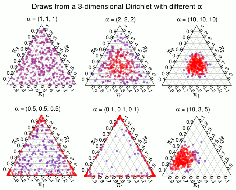
When $\alpha = (1,1,1)$ the distribution is uniform, any combination of $(\pi_1,\pi_2,\pi_3)$ that forms a proportion is equally likely. But as $\alpha \rightarrow (0, 0, 0)$ the density is “pushed” towards the edges of the triangle making proportions like $(033, 0.33, 0.33)$ very unlikely in favor of proportions like $(0.9, 0.1, 0.0)$ and $(0.0, 0.5, 0.5)$. We want a Dirichlet distribution of this latter type, a distribution that puts most of the density over combination of proportions where most of the $\pi$s are zero and only few $\pi$s are large. Using this type of prior will make the model consider it very likely apriori that most of the data $x$ is produced from a small number of the possible values $d$. And in the limit when $\alpha = (0, \ldots, 0)$ the model will consider it impossible that $x$ takes on more than one value in $d$ unless there is data that shows otherwise. So using a $\text{Dirichlet}(0_1, \ldots, 0_K)$ over $\pi$ achieves the hallmark of the bootstrap, that the model only considers values already seen in the data as possible. The full model is then:

$$ \begin{align*} &\begin{array}{l} x_i \leftarrow d_{k_i}\\ k_i \sim \text{Categorical}(\pi) \end{array} \bigg\} ~ \text{for $i$ in $1..N$} \\ &\pi \sim \text{Dirichlet}(0_1, \ldots, 0_K) \end{align*} $$

So is this a reasonable model? Surprise, surprise: It depends. For binary data, $d = (0, 1)$, the Bayesian bootstrap is the same as assuming $x_i \sim \text{Bernoulli}(p)$ with an improper $p \sim \text{Beta(0,0)}$ prior. A completely reasonable model, if you’re fine with the non-informative prior. Similarly it reduces to a categorical model when $d$ are a number of categories. For integer data, like count data, the Bayesian bootstrap implies treating each possible value as its own isolated category, disregarding any prior information regarding a relation between the values (such that three eggs are more that two eggs, but less than four). For continuous data the assumptions of the bootstrap feel a bit weird because we are leaving out obvious information: That the data is actually continuous and that a data point of, say, 3.1 should inform the model that values that are close (like 3.0 and 3.2) are also more likely.

If you don’t include useful prior information in a model you will have to make up with information from another source in order to get as precise estimates. This source is often the data, which means you might need relatively more data when using the bootstrap. You might say that the bootstrap makes very naïve assumptions, or perhaps very conservative assumptions, but to say that the bootstrap makes no assumptions is wrong. It makes really strong assumptions: The data is discrete and values not seen in the data are impossible.

So let’s take the Bayesian bootstrap for a spin by using the cliché example of inferring a mean. I’ll compare it with using the classical non-parametric bootstrap and a Bayesian model with flat priors that assumes that the data is normally distributed. To implement the Bayesian bootstrap I’m using this handy script published at R-snippets.

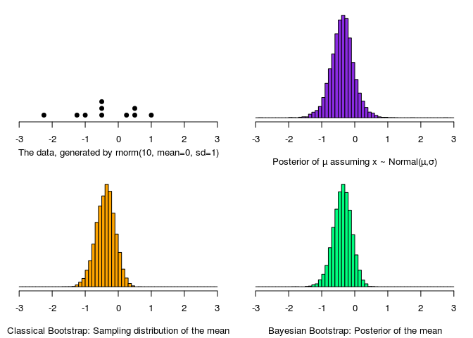
Compared to the “gold standard” of the Normal Bayesian model both the classical and the Bayesian bootstrap have shorter tails, otherwise they are pretty spot on. Note also that the two bootstrap distributions are virtually identical. Here, and in the model definition, the data $x_i$ was one-dimensional, but it’s easy to generalize to bi-variate data by replacing $x_i$ with $(x_{1i}, x_{2i})$ (and similar for multivariate data).

I feel that, in the case of continuous data, the specification of the Bayesian bootstrap as given above is a bit strange. Sure, “all data as observed are discrete”, but it would be nice with a formulation of the Bayesian bootstrap that fits more natural with continuous data.

The bootstrap as a Bayesian model, version two

The Bayesian bootstrap can be characterized differently than the version given by Rubin (1981). The two versions result in the exact same inferences but I feel that the second version given below is a more natural characterization when the data is assumed continuous. It is also very similar to a Dirichlet process which means that the connection between the Bayesian bootstrap and other Bayesian non-parametric methods is made clearer.

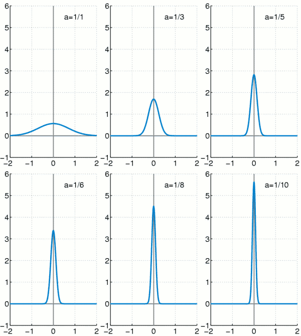
This second characterization requires two more distributions to get going: The Dirac delta distribution and the geometric distribution. The Dirac delta distribution is so simple that is almost doesn’t feel like a distribution at all. It is written $x \sim \delta(x_0)$ and is a probability distribution with zero density except at $x_0$. Assuming, say, $x \sim \delta(5)$ is basically the same as saying that $x$ is fixed at 5. The delta distribution can be seen as a Normal distribution where the standard deviation is approaching zero, as this animation off Wikipedia nicely demonstrates:

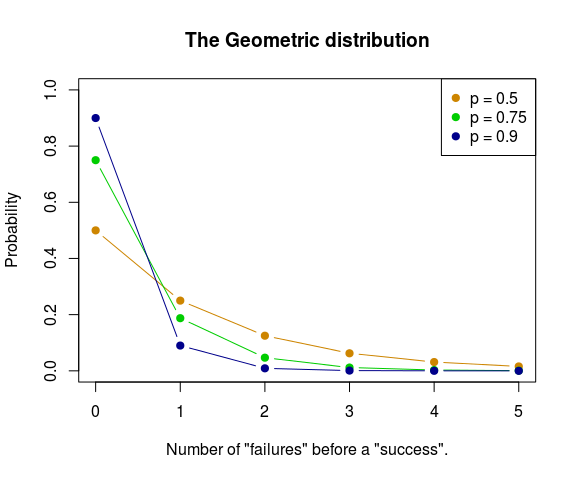
The geometric distribution is the distribution over how many “failures” there are in a number of Bernoulli trials before there is a success, where the one parameter is $p$, the relative frequency of success. Here are some geometric distributions with different $p$:

We’ll begin this second version of the Bayesian bootstrap by assuming that the data $x = (x_1, \ldots, x_N)$ is distributed as a mixture of $\delta$ distributions with $M$ components, where $\mu = (\mu_1, \ldots, \mu_M)$ are the parameters of the $\delta$s. The $\mu$s are given a flat $\text{Uniform}(-\infty,\infty)$ distribution and the mixture probabilities $\pi = (\pi_1, \ldots, \pi_M)$ are again given a $\text{Dirichlet}(0_1, \ldots,0_M)$ distribution. Finally, $M$, the number of component distributions in the mixture, is given a $\text{Geometric}(p)$ distribution where $p$ is close to 1. Here is the full model:

$$\begin{align*} &\begin{array}{l} x_i \sim \delta(\mu_{k_i}) \\ k_i \sim \text{Categorical}(\pi) \end{array} \bigg\} &\text{for $i$ in $1..N$} \\ &\mu_j \sim \text{Uniform}(-\infty,\infty) &\text{for $j$ in $1..M$} \\ &\pi \sim \text{Dirichlet}(0_1, \ldots, 0_M) & ~ \\ &M \sim \text{Geometric}(p) &\text{with $p$ close to 1} \end{align*}$$

There is more going on in this version of the Bayesian bootstrap, but what the model is basically assuming is this: The data comes from a limited number of values (the $\mu$s) where each value can be anywhere between $-\infty$ and $\infty$. A data point ($x_i$) comes from a specific value ($\mu_j$) with a probability ($\pi_j$), but what these probabilities $(\pi_1, \ldots, \pi_M)$ are is very uncertain (due to the Dirichlet prior). The only part that remains is how many values ($M$) the data is generated from. This is governed by the Geometric distribution where $p$ can be seen as the probability that the current number of values ($M$) is the maximum number needed. When $p \approx 1$ the number of values will be kept to a minimum unless there is overwhelming evidence that another value is needed. But since the data is distributed as a pointy Dirac $\delta$ distribution a set of data of, say, $x = (3.4, 1.2, 4.1)$ is overwhelming evidence of that $M$ is at least 3 as there is no other possible way $x$ could take on three different values.

So, I like this characterization of the Bayesian bootstrap because it connects to Bayesian non-parametrics and it is more easy for me to see how it can be extended. For example, maybe you think the Dirac $\delta$ distribution is unreasonably sharply peaked? Then just swap it for a distribution that better matches what you know about the data (a Normal distribution comes to mind). Do you want to include prior information regarding the location of the data? Then swap the $\text{Uniform}(-\infty,\infty)$ for something more informative. Is it reasonable to assume that there are between five and ten clusters / component distributions? Then replace the geometric distribution with a $\text{Discrete-Uniform}(5, 10)$. And so on. If you want to go down this path you should read up on Bayesian non-parametrics (for example, this tutorial). Actually, for you that are already into this, a third characterization of the Bayesian bootstrap is as a Dirichlet process with $\alpha \rightarrow 0$ ( Clyde and Lee, 2001).

Again, the bootstrap is a very “naïve” model. A personification of the bootstrap would be a savant learning about peoples lengths, being infinitely surprised by each new length she observed. “Gosh! I knew people can be 165 cm or 167 cm, but look at you, you are 166 cm, who knew something like that was even possible?!”. However, while it will take many many examples, Betty Bootstrap will eventually get a pretty good grip on the distribution of lengths in the population. Now that I’ve written at length about the Bayesian bootstrap, what is its relation with the classical non-parametric bootstrap?

Three ways the classical bootstrap is a special case of the Bayesian bootstrap

I can think of three ways the classical bootstrap of Efron (1979) can be considered a special case of the Bayesian bootstrap. Just because the classical bootstrap can be considered a special case doesn’t mean it is necessarily “better” or “worse”. But, from a Bayesian perspective, I don’t see how the classical bootstrap has any advantage over the Bayesian (except for being computationally more efficient, easier to implement and perhaps more well know by the target audience of the analysis…). So in what way is the classical bootstrap a special case?

1. It’s the Bayesian bootstrap but with discrete weights

When implemented by Monte Carlo methods, both the classical and Bayesian bootstrap produces draws that can be interpreted as probability weights over the input data. The classical bootstrap does this by “sampling with replacement” which is another way of saying that the weights $\pi = (\pi_1, \ldots, \pi_n)$ for the $N$ data points are created by drawing counts $c = (c_1, \ldots, c_N)$ from a $\text{Multinomial}(p_1, \ldots, p_N)$ distribution with $N$ trials where all $p$s = $1/N$. Each count is then normalized to create the weights: $\pi_i = c_i / N$. For example, say we have five data points, we draw from a Multinomial and get $(0, 2, 2, 1, 0)$ which we normalize by dividing by five to get the weights $(0, 0.4, 0.4, 0.2, 0)$. With the Bayesian bootstrap, the $N$ probability weights can instead be seen as being drawn from a flat $\text{Dirichlet}(1_1, \ldots, 1_N)$ distribution. This follows directly from the model definition of the Bayesian bootstrap and an explanation for why this is the case can be found in Rubin (1981). For example, for our five data points we could get weights $(0, 0.4, 0.4, 0.2, 0)$ or $(0.26,0.1,0.41,0.01,0.22)$.

Setting aside philosophical differences, the only difference between the two methods is in how the weights are drawn, and both methods result in very similar weight distributions. The mean of either weight distributions is the same, each probability weight $\pi_j$ has a mean of $1/N$ both when using the Multinomial and the Dirichlet. The variance of the weights are almost the same. For the classical bootstrap the variance is $(n + 1) / n$ times the variance for the bootstrap weights and this difference grows small very quickly as $n$ gets large. These similarities are presented in Rubin’s original paper on the Bayesian bootstrap and discussed in a friendly manner by Friedman, Hastie and Tibshirani (2009) on p. 271.

From a Bayesian perspective I find three things that are slightly strange with how the weights are drawn in the classical bootstrap (but from a sampling distribution perspective it makes total sense, of course):

1. Why have discrete steps for the probability weights, where the granularity of the discretization changes with the sample size?
2. Why allow weights of 0% for a data point? If anything, we know that the process actually can produce all the values of the input data and therefore a weight of 0% is not logically possible.
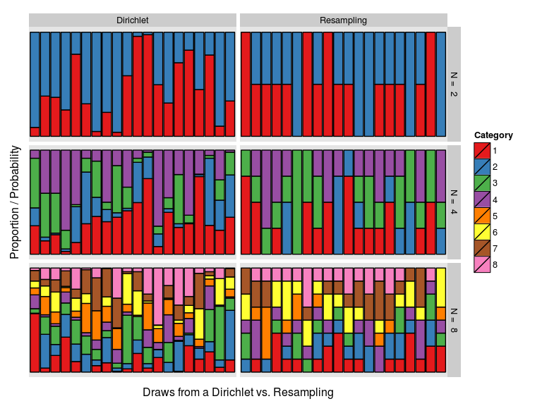
3. The classical bootstrap is more likely to draw weight vectors that are even. For example, in the 2D case the weight vector $\pi = (0.5, 0.5)$ is selected with 50% probability, while the weight vectors $\pi = (1.0, 0.0)$ and $\pi = (0.0, 1.0)$ are selected with only 25% probability. Why this bias? The Bayesian bootstrap has no such bias, any combination of weights is equally likely.

Let’s try to visualize the difference between the two versions of the bootstrap! Below is a graph where each colored column is a draw of probability weights, either from a Dirichlet distribution (to the left) or using the classical resampling scheme (to the right). The first row shows the case with two data points ($N = 2$). Here the difference is large, draws from the Dirichlet vary smoothly between 0% and 100% while the resampling weights are either 0%, 50% or 100%, with 50% being roughly twice as common. However, as the number of data points increases, the resampling weights vary more smoothly and become more similar to the Dirichlet weights.

This difference in how the weights are sampled can also be seen when comparing the resulting distributions over the data. Below, the classical and the Bayesian bootstrap are used to infer a mean when applied to two, four and eight samples from a $\text{Normal(0, 1)}$ distribution. At $N = 2$ the resulting distributions look very different, but they look almost identical already at $N = 8$. (One reason for this is because we are inferring a mean, other statistics could require many more data points before the two bootstrap methods “converge”.)

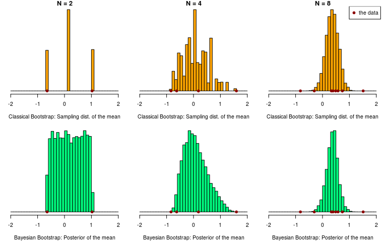
It is sometimes written that “the Bayesian bootstrap can be thought of as a smoothed version of the Efron bootstrap” (Lancaster, 2003), but you could equally well think of the classical bootstrap as a rough version of the Bayesian bootstrap! Nevertheless, as $N$ gets larger the classical bootstrap quickly becomes a good approximation to the Bayesian bootstrap, and similarly the Bayesian bootstrap quickly becomes a good approximation to the classical one.

2. It’s the posterior mean of the Bayesian bootstrap

Above we saw a connection between the Bayesian bootstrap and the classical bootstrap procedure, that is, using sampling with replacement to create a distribution over some statistic. But you can also show the connection between the models underlying both methods. For the classical bootstrap the underlying model is that the distribution of the data is the distribution of the population. For the Bayesian bootstrap the values in the data define the support of the predictive distribution, but how much each value contributes to the predictive depends on the probability weights which are, again, distributed as a $\text{Dirichlet}(1, \ldots, 1)$ distribution. If we discard the uncertainty in this distribution by taking a point estimate of the probability weights, say the posterior mean, we end up with the following weights: $(1/N, \ldots, 1/N)$. That is, each data point contributes equally to the posterior predictive, which is exactly the assumption of the classical bootstrap. So if you just look at the underlying models, and skip that part where you simulate a sampling distribution, the classical bootstrap can be seen as the posterior mean of the Bayesian bootstrap.

3. It’s the Bayesian bootstrap (version two) but with a Dirichlet(∞, …, ∞) prior

The model of the classical bootstrap can also be put as a special case of the model for the Bayesian bootstrap, version two. In that model the probability weights $\pi = (\pi_1, \ldots, \pi_M)$ were given an uninformative $\text{Dirichlet}(\alpha_1, \ldots,\alpha_M)$ distribution with $\alpha = 0$. If we would increase $\alpha$ then combinations with more equal weights would become successively more likely:

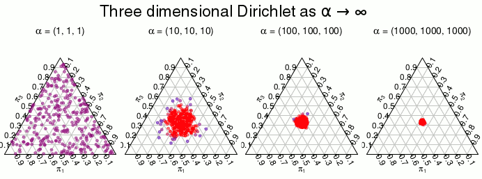
In the limit of $\alpha \rightarrow \infty$, the only possible weight becomes $\pi = (1/M, \ldots, 1/M)$, that is, the model is “convinced” that all seen values contribute exactly equally to the predictive distribution. That is, the same assumption as in the classical bootstrap! Note that this only works if all seen data points are unique (or assumed unique) as would most often be the case with continuous data.

Let’s apply the $\text{Dirichlet}(\infty, \ldots,\infty)$ version of the classical bootstrap to 30 draws from a $\text{Normal}(0, 1)$ distribution. The following animation then illustrates the uncertainty by showing draws from the posterior predictive distribution:

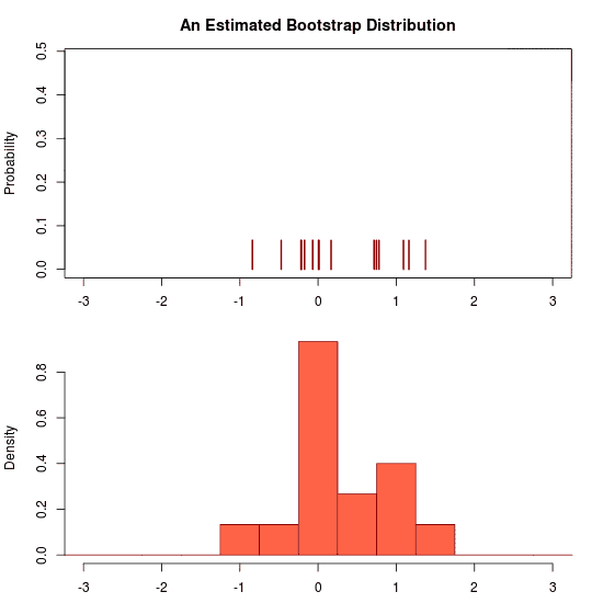
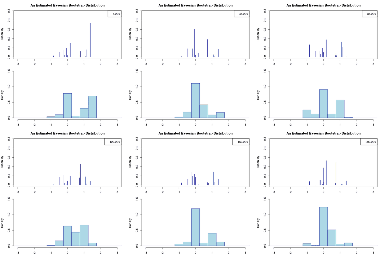
He he, just trolling you. Due to the $\text{Dirichlet}(\infty, \ldots,\infty)$ prior there is no uncertainty at all regarding the predictive distribution. Hence the “animation” is a still image. Let’s apply the Bayesian bootstrap to the same data. The following (actual) animation shows the uncertainty by plotting 200 draws from the posterior predictive distribution:

Some final thoughts

I like the non-parametric bootstrap, both the classical and the Bayesian version. The bootstrap is easy to explain, easy to run and often gives reasonable results (despite the somewhat weird model assumptions). From a Bayesian perspective it is also very natural to view the classical Bootstrap as an approximation to the Bayesian bootstrap. Or as Friedman et al (2009, p. 272) put it:

In this sense, the bootstrap distribution represents an (approximate) nonparametric, noninformative posterior distribution for our parameter. But this bootstrap distribution is obtained painlessly — without having to formally specify a prior and without having to sample from the posterior distribution. Hence we might think of the bootstrap distribution as a “poor man’s” Bayes posterior. By perturbing the data, the bootstrap approximates the Bayesian effect of perturbing the parameters, and is typically much simpler to carry out.

You can also view the Bayesian bootstrap as a “poor man’s” model. A model that makes very weak assumptions (weak as in uninformative), but that can be used in case you don’t have the time and resources to come up with something better. However, it is almost always possible to come up with a model that is better than the bootstrap, or as Donald B. Rubin (1981) puts it:

[…] is it reasonable to use a model specification that effectively assumes all possible distinct values of X have been observed?

No, probably not.

References

Alfaro, M. E., Zoller, S., & Lutzoni, F. (2003). Bayes or bootstrap? A simulation study comparing the performance of Bayesian Markov chain Monte Carlo sampling and bootstrapping in assessing phylogenetic confidence. ‘Molecular Biology and Evolution, 20(2), 255-266. pdf

Clyde, M. A., & Lee, H. K. (2001). Bagging and the Bayesian bootstrap. In Artificial Intelligence and Statistics. pdf

Efron, B. (1979). Bootstrap methods: another look at the jackknife. The annals of Statistics, 1-26. pdf

Friedman, J., Hastie, T., & Tibshirani, R. (2009). The Elements of Statistical Learning: Data Mining, Inference, and Prediction. Springer Series in Statistics. Freely available at https://www-stat.stanford.edu/~tibs/ElemStatLearn/ .

Gershman, S. J., & Blei, D. M. (2012). A tutorial on Bayesian nonparametric models. Journal of Mathematical Psychology, 56(1), 1-12. pdf

Lancaster, T. (2003). A note on bootstraps and robustness. SSRN 896764. pdf

Rubin, D. B. (1981). The Bayesian Bootstrap. The annals of statistics, 9(1), 130-134. pdf