I recently wrapped up a version of my R function for easy Bayesian bootstrappin’ into the package bayesboot. This package implements a function, also named bayesboot, which performs the Bayesian bootstrap introduced by Rubin in 1981. The Bayesian bootstrap can be seen as a smoother version of the classical non-parametric bootstrap, but I prefer seeing the classical bootstrap as an approximation to the Bayesian bootstrap :)

The implementation in bayesboot can handle both summary statistics that works on a weighted version of the data (such as weighted.mean) and that works on a resampled data set (like median). As bayesboot just got accepted on CRAN you can install it in the usual way:

install.packages("bayesboot")

You’ll find the source code for bayesboot on GitHub. If you want to know more about the model behind the Bayesian bootstrap you can check out my previous blog post on the subject and, of course, the original paper by Rubin (1981).

A simple example of bayesboot in action

As in a previous post on the Bayesian bootstrap, here is again a Bayesian bootstrap analysis of the mean height of American presidents using the heights of the last ten presidents:

# Heights of the last ten American presidents in cm (Kennedy to Obama).
heights <- c(183, 192, 182, 183, 177, 185, 188, 188, 182, 185)

The bayesboot function needs, at least, a vector of data and a function implementing a summary statistic. Here we have the data height and we’re going with the sample mean as our summary statistic:

library(bayesboot)
b1 <- bayesboot(heights, mean)

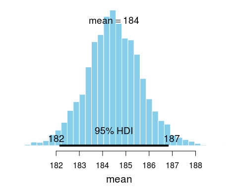
The resulting posterior distribution over probable mean heights can now be plotted and summaryized:

summary(b1)

## Bayesian bootstrap
## 
## Number of posterior draws: 4000 
## 
## Summary of the posterior (with 95% Highest Density Intervals):
##  statistic  mean    sd hdi.low hdi.high
##         V1 184.5 1.181   182.1    186.8
## 
## Quantiles:
##  statistic q2.5%  q25% median  q75% q97.5%
##         V1 182.2 183.7  184.5 185.3  186.9
## 
## Call:
##  bayesboot(data = heights, statistic = mean)

plot(b1)

A shout-out to Mike Meredith and John Kruschke who implemented the great BEST and HDInterval packages which summary and plot utilizes. Note here that the point mean in the summary and plot above refers to the mean of the posterior distribution and not the sample mean of any presidents.

While it is possible to use a summary statistic that works on a resample of the original data, it is more efficient to use a summary statistic that works on a reweighting of the original dataset. So instead of using mean as above it would be better to use weighted.mean, like this:

b2 <- bayesboot(heights, weighted.mean, use.weights = TRUE)

The result will be almost the same as before, but the above will be somewhat faster to compute.

The result of a call to bayesboot will always result in a data.frame with one column per dimension of the summary statistic. If the summary statistic does not return a named vector the columns will be called V1, V2, etc. The result of a bayesboot call can be further inspected and post processed. For example:

# Given the model and the data, this is the probability that the mean
# heights of American presidents is above the mean heights of
# American males as given by www.cdc.gov/nchs/data/series/sr_11/sr11_252.pdf
mean( c(b2$V1 > 175.9, TRUE, FALSE) )

## [1] 0.9998

Comparing two groups

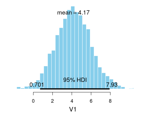
If we want to compare the means of two groups, we will have to call bayesboot twice with each dataset and then use the resulting samples to calculate the posterior difference. For example, let’s say we have the heights of the opponents that lost to the presidents in height the first time those presidents were elected. Now we are interested in comparing the mean height of American presidents with the mean height of presidential candidates that lost.

# The heights of opponents of American presidents (first time they were elected).
# From Richard Nixon to John McCain
heights_opponents <- c(182, 180, 180, 183, 177, 173, 188, 185, 175)

# Running the Bayesian bootstrap for both datasets
b_presidents <- bayesboot(heights, weighted.mean, use.weights = TRUE)
b_opponents  <- bayesboot(heights_opponents, weighted.mean, use.weights = TRUE)

# Calculating the posterior difference and converting back to a 
# bayesboot object for pretty plotting.
b_diff <- as.bayesboot(b_presidents - b_opponents)
plot(b_diff)

So there is some evidence that winning presidents are a couple of cm taller than loosing opponents. (Though, I must add that it is quite unclear what the purpose really is of analyzing the heights of presidents and opponents…)

More information

The README and documentation of bayesboot contains more examples. If you find any bugs or have suggestions for improvements consider submitting an issue on GitHub.

References

Rubin, D. B. (1981). The Bayesian bootstrap. The annals of statistics, 9(1), 130–134. link to paper