This January I played the most intriguing computer game I’ve played in ages: The Return of the Obra Dinn. Except for being a masterpiece of murder-mystery storytelling it also has the most unique art-style as it only uses black and white pixels. To pull this off Obra Dinn makes use of image dithering: the arrangement of pixels of low color resolution to emulate the color shades in between. Since the game was over all too quickly I thought I instead would explore how basic image dithering can be implemented in R. If old school graphics piques your interest, read on! There will be some grainy looking ggplot charts at the end.

(The image above is copyright Lucas Pope and is the title screen of The Return of the Obra Dinn)

Horatio Nelson in black and white

Image dithering tries to solve the problem that you want to show an image with many shades of color, but your device can only display a much smaller number of colors. This might sound like a silly problem now, but was a very real problem in the early days of computers. For example, the original Mac could only display black and white pixels, not even any shades of grey!

So let’s do some image dithering in R! The Return of Obra Dinn takes place on an early 19th century East Indiaman ship, so let’s use something related as an example image. Why not use a low-resolution painting of Vice Admiral Horatio Nelson (1758 - 1805) the British officer who defeated the French and Spanish navies during the battle of Trafalgar. To read in the image I will use the imager package.

library(imager)
nelson <- load.image("horatio_nelson.jpg")
nelson

## Image. Width: 199 pix Height: 240 pix Depth: 1 Colour channels: 3

The imager package is a really useful package when you want to manipulate (and mess with) images directly in R. The nelson object is now a cimg object, which is basically an array with dimensions Width, Height, Depth (a time dimension, if you have a series of images), and Color channels. More importantly, cimg objects can be plotted:

plot(nelson)

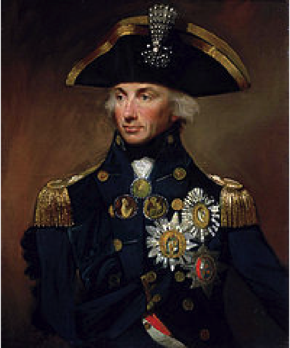
As an example, I’m going to do black-and-white dithering so let’s remove the color and any transparency (called “alpha” here) from the image.

nelson_gray <- grayscale( rm.alpha(nelson) )
plot(nelson_gray)

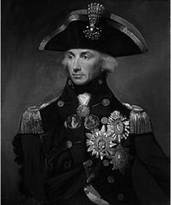
Now let’s imagine that we would want to display this image using only black and white pixels. Before getting to the dithering, what would the simplest method be to achieve this? Well, we could just threshold the image. A pixel with value 0.0 (fully black) to 0.5 are made black, and pixels with values above 0.5 are set to white (1.0). This is easy to do as nelson_gray can be treated as a matrix:

nelson_threshold <- nelson_gray > 0.5
plot(nelson_threshold)

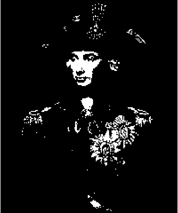
So, while the image looks kind of cool, it has lost a lot of nuance as large parts of it are now completely black. So how to fake shades of gray using only black and white pixels? Well, you can dither the image, that is, add some noise to the image as you reduce the number of colors. Let’s start by trying out the most basic kind of noise: White noise, here created using the runif function:

rand_matrix <- matrix(
  data = runif(length(nelson_gray)), 
  ncol = ncol(nelson_gray), nrow=nrow(nelson_gray))
rand_cimg <- as.cimg(rand_matrix)
plot(rand_cimg)

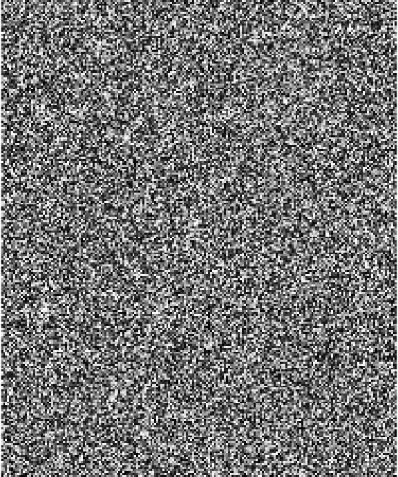
Each pixel in rand_cimg is a value from 0.0 to 1.0 and we can now use rand_cimg when thresholding instead of the static 0.5. If you try out many different noise images then every black and white pixel will on average have the same value as the original grayscale pixel. This sounds like a good property, but let’s see how it looks with the current rand_cimg:

nelson_rand <- nelson_gray > rand_cimg
plot(nelson_rand)

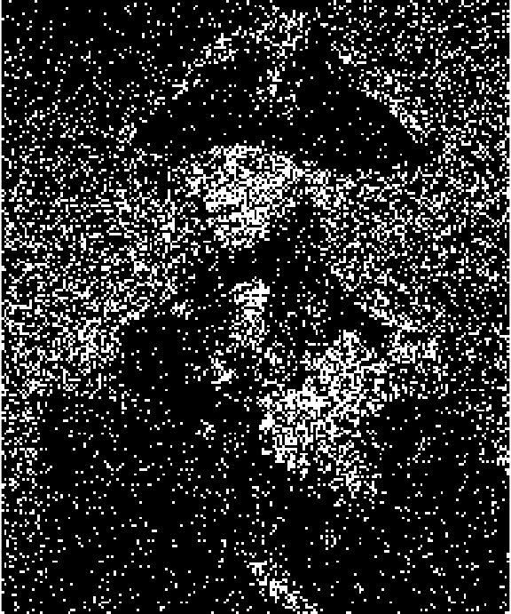
To be correct on average doesn’t help much, in practice, we get a very noisy Nelson. But if you squint you can now see shades of gray in the picture, at least. Random noise is just too random, but maybe we can get better dithering by adding less random noise. What about a checker pattern?

checker_pattern <- rbind(c(1/3, 2/3), 
                         c(2/3, 1/3))
plot(as.cimg(checker_pattern))

The pattern above uses cutoffs of 1/3 and 2/3, so Nelson-pixels that gets compared to a darker 1/3-pixel will be more likely to go white and Nelson-pixels that are compared to a lighter 2/3-pixel will tend to go black. Let’s scale this patter to Nelson-size.

# rep_mat takes a matrix (mat) and tiles it so that the resulting
# matrix has size nrow_out x ncol_out.
# It's basically a 2d version of rep()
rep_mat <- function(mat, nrow_out, ncol_out) {
  mat[rep(seq_len(nrow(mat)), length.out = nrow_out),
      rep(seq_len(ncol(mat)), length.out = ncol_out)]
}

checker_cimg <- as.cimg(rep_mat(checker_pattern, nrow(nelson_gray), ncol(nelson_gray)))
plot(checker_cimg)

And let’s do the thresholding with this new checker pattern:

nelson_checker <- nelson_gray > checker_cimg
plot(nelson_checker)

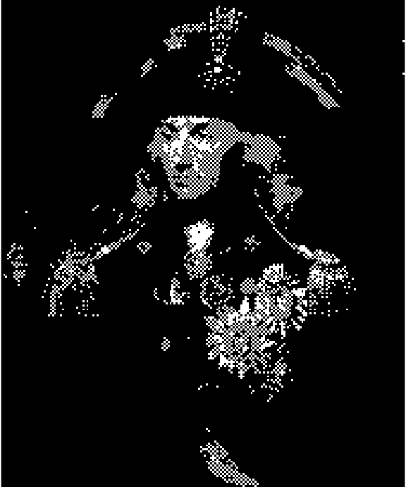
Well, it’s not good, but it kind of looks like we got at least one shade of gray now compared to using the static 0.5. Actually, that’s exactly what we got! We can see that by taking a smooth gradient…

gradient <- as.cimg( rep(seq(0, 1, 0.01), 101), x=101, y=101)
plot(gradient)

… and thresholding with the checker pattern:

checker_cimg <- as.cimg(rep_mat(checker_pattern, 
                                nrow(gradient), ncol(gradient)))
gradient_checker <- gradient > checker_cimg
plot(gradient_checker)

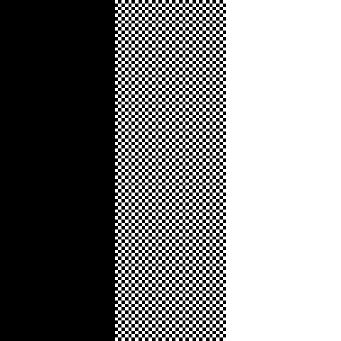
This gives us three columns: black, “checker-gray”, and white. So, using the checker pattern we can achieve some more nuance than with simple thresholding. Is there perhaps an even better pattern that allows for even more nuance?

Better patterns, Bayer patterns

Yes, there is! The classical pattern used in many image dithering implementations is the Bayer pattern (or Bayer matrix) named after it’s inventor Bryce Bayer. It’s an evolution of the checker pattern defined for matrices of size 2×2, 4×4, 8×8, etc. The exact construction and properties of the Bayer matrix are well described in the Wikipedia article but here is how to create it in R and how it looks:

# Calculates a non-normalized Bayer pattern matrix of size 2^n
recursive_bayer_pattern <- function(n) {
  if(n <= 0) {
    return(matrix(0))
  }
  m <- recursive_bayer_pattern(n - 1)
  rbind(
    cbind(4 * m + 0, 4 * m + 2),
    cbind(4 * m + 3, 4 * m + 1))
}

# Returns a Bayer pattern of size 2^n normalized so all values
# are between 0.0 and 1.0.
normalized_bayer_pattern <- function(n) {
  pattern <- recursive_bayer_pattern(n)
  (1 + pattern) / ( 1 + length(pattern) )
}

par(mfcol = c(1, 3), mar = c(0, 0, 2, 1), ps = 18)
plot(as.cimg(normalized_bayer_pattern(1)), main = "Bayer 2×2")
plot(as.cimg(normalized_bayer_pattern(2)), main = "Bayer 4×4")
plot(as.cimg(normalized_bayer_pattern(3)), main = "Bayer 8×8")

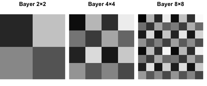
Basically, a Bayer matrix contains as many shades of gray it’s possible to fit in there, and the shades are as spread out as possible. Let’s see how a 4x4 Bayer matrix transforms the smooth gradient:

bayer_cimg <- as.cimg(rep_mat(normalized_bayer_pattern(2), 
                              nrow(gradient), ncol(gradient)))
gradient_bayer <- gradient > bayer_cimg
plot(gradient_bayer)

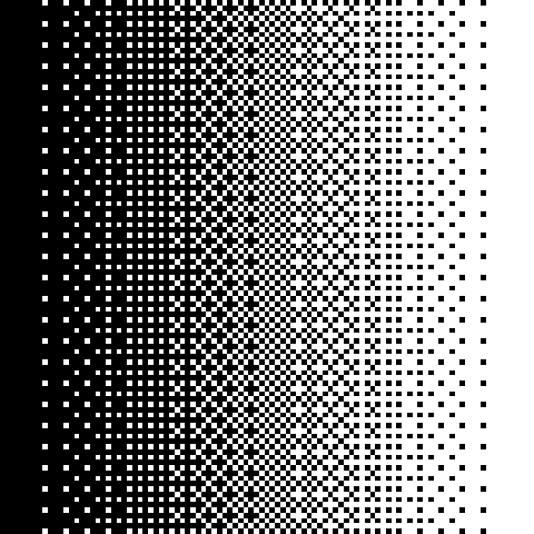
Pretty smooth! We get the classical “crosshatch” patterns reminiscent of last-century computer graphics. Let’s give Admiral Nelson the same treatment:

bayer_matrix <- rep_mat(normalized_bayer_pattern(2), 
                        nrow(nelson_gray), ncol(nelson_gray))
bayer_cimg <- as.cimg(bayer_matrix)
nelson_bayer <- nelson_gray > bayer_cimg
plot(nelson_bayer)

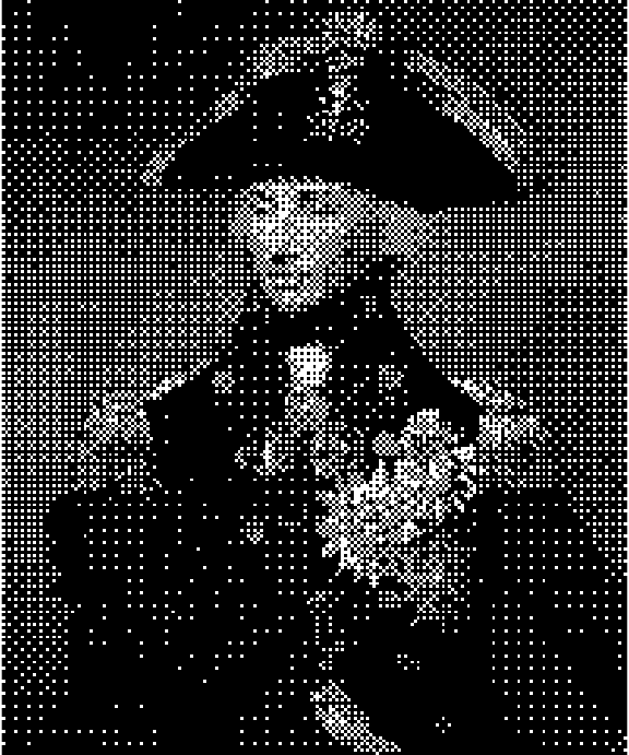
Now he looks doubly old-school. So far I’ve only worked with grayscale images and black-and-white dithering, but we can quickly hack together some color dithering by just performing the dither thresholding on one color channel at a time.

nelson_bayer_color <- nelson
for(rgb_i in 1:3) {
  color_channel <- nelson_bayer_color[ , , 1, rgb_i, drop = FALSE]
  nelson_bayer_color[ , , 1, rgb_i] <- color_channel > bayer_cimg
}
plot(nelson_bayer_color)

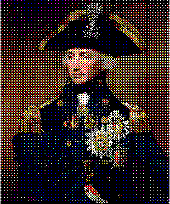
This method does not generalize to arbitrary color scales, but I still think it looks pretty cool!

Image dithering ggplots in R

Finally, I’ll show you how to dither some ggplots. Below is most of the code above wrapped up into functions:

# rep_mat takes a matrix (mat) and tiles it so that the resulting
# matrix has size nrow_out × ncol_out.
# It's basically a 2d version of rep()
rep_mat <- function(mat, nrow_out, ncol_out) {
  mat[rep(seq_len(nrow(mat)), length.out = nrow_out),
      rep(seq_len(ncol(mat)), length.out = ncol_out)]
}

# Calculates a Bayer pattern matrix of size 2^n
# Source: https://gist.github.com/MehdiNS/bd41bbc6db780c9409157d35d331ac80
recursive_bayer_pattern <- function(n) {
  if(n <= 0) {
    return(matrix(0))
  }
  m <- recursive_bayer_pattern(n - 1)
  rbind(
    cbind(4 * m + 0, 4 * m + 2),
    cbind(4 * m + 3, 4 * m + 1))
}

# Returns a Bayer pattern of size 2^n normalized so all values
# are between 1 / (m + 1) and m / (m + 1) where m is the number 
# of elements in the 2^n × 2^n matrix.
normalized_bayer_pattern <- function(n) {
  pattern <- recursive_bayer_pattern(n)
  (1 + pattern) / ( 1 + length(pattern) )
}

# Returns a  nrow_out × ncol_out cimg image repeatig a 2×2 Bayer pattern
rep_bayer_cimg <- function(nrow_out, ncol_out) {
  bayer_matrix <- rep_mat(normalized_bayer_pattern(2), nrow_out, ncol_out)
  as.cimg(bayer_matrix)  
}

# Transforms a cimg image into a dithered black and white image
img_to_bayer_bw <- function(img) {
  img <- grayscale(rm.alpha(img))
  bayer_cimg <- rep_bayer_cimg(nrow(img), ncol(img))
  img >= bayer_cimg
}
 
# Transforms a cimg image into a dithered color image with 8 colors.
img_to_bayer_color <- function(img) {
  img <- rm.alpha(img)
  bayer_cimg <- rep_bayer_cimg(nrow(img), ncol(img))
  for(rgb_i in 1:3) {
    color_channel <- img[ , , 1, rgb_i, drop = FALSE]
    img[ , , 1, rgb_i] <- color_channel >= bayer_cimg
  }
  img
} 

Let’s then create the ggplot we will transform.

library(ggplot2)
ggplot(mtcars, aes(factor(cyl), mpg, fill = factor(cyl))) + 
  geom_violin(color = "black") +
  theme_classic() + 
  theme(axis.text= element_text(colour="black"))

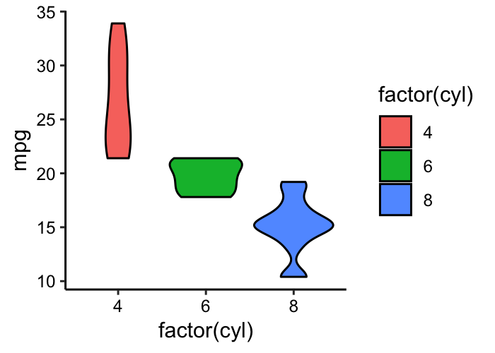
Then we’ll turn it into a low res cimg image.

# This function is a hack to read in a ggplot2 plot as a cimg image 
# by saving it as a png to disk and reading it back in.
ggplot_to_cimg <- function(width, height, dpi) {
  tmp_fname <- tempfile(fileext = ".png")
  ggsave(tmp_fname, width = width, height = height, dpi = dpi, antialias = "none")
  load.image(tmp_fname)
}

plot_img <- ggplot_to_cimg( width = 3, height = 2, dpi = 140)
plot(plot_img)

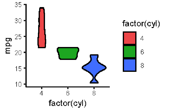
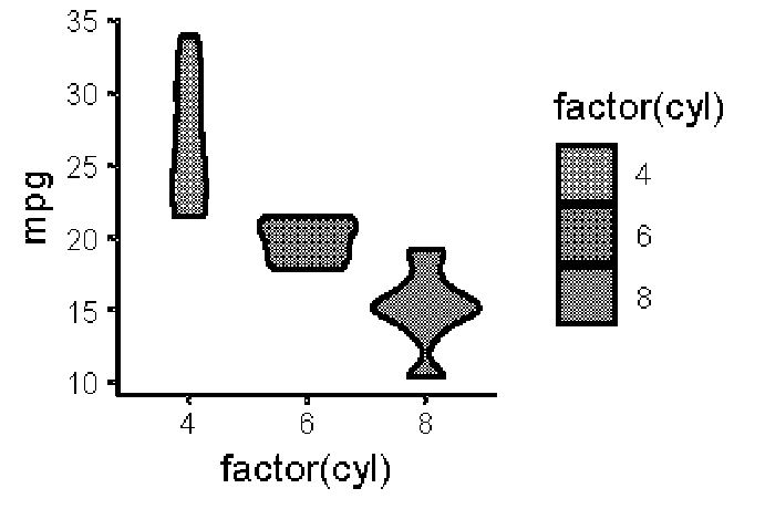
Finally, we can turn it into a retro-dithered black and white plot…

plot( img_to_bayer_bw(plot_img) )

…or a dithered eight-color plot.

plot( img_to_bayer_color(plot_img) )

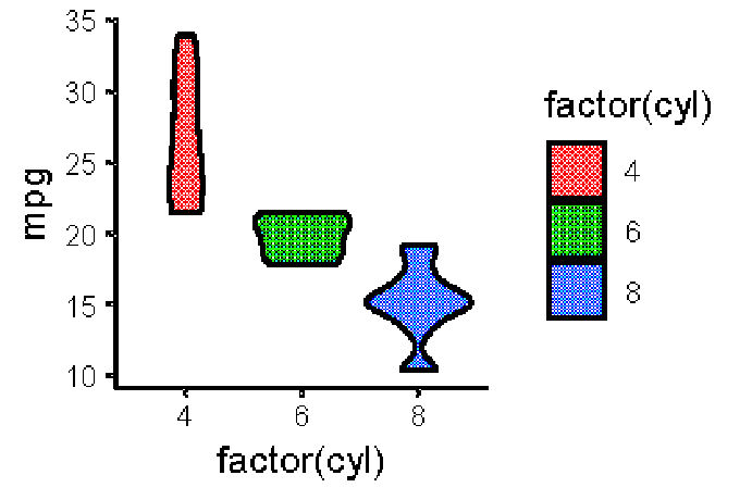
Something for your next retro inspired presentation, maybe? If you want to have full control over your image dithering it would probably be more convenient to post-process your plots using an image editor, such as the free and open source GIMP rather than to do it directly in R.

This post has covered basic image dithering in R and, to be more specific, it has covered ordered dithering. There is also error-diffusion dithering which works in a rather different way. But that’s for another time. Now I’m going to go back to mourning that I’ve already finished The Return of the Obra Dinn.