Hello stranger, and welcome! 👋😊
I'm Rasmus Bååth, data scientist, engineering manager, father, husband, tinkerer,
tweaker, coffee brewer, tea steeper, and, occasionally, publisher of stuff I find
interesting down below👇
For some reason someone dropped a pamphlet advertising SPSS for Windows 3.0 in my mail box at work. This means that the pamphlet, and the advertised version of SPSS, should be at least 20 years old! These days I’m happily using R for everything but if I was going to estimate any models 20 years ago SPSS actually looked quite OK. In the early 90s my interests in computing were more related to making Italian plumbers rescue princesses than estimating regression models.
The pamphlet is quite fun to read, there are many things in it that feels really out of date and which shows how much have happened in computing in the last 20 years. Let me show you some of the highlights!
Here is a picture from the pamphlet of an SPSS session in action:
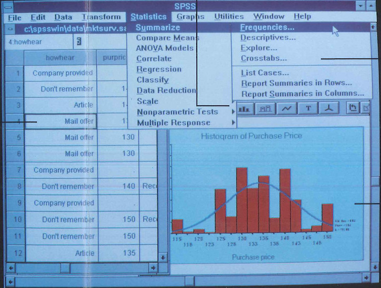
Actually it still looks very similar to the SPSS I saw my colleague use yesterday, so maybe not that much have changed in 20 years… Well let’s look at the hardware requirements:
So in
the last post I showed how to run the Bayesian counterpart of Pearson’s correlation test by estimating the parameters of a bivariate normal distribution. A problem with assuming normality is that the normal distribution isn’t robust against outliers. Let’s see what happens if we take the data from
the last post with the finishing times and weights of the runners in the men’s 100 m semi-finals in the 2013 World Championships in Athletics and introduce an outlier. This is how the original data looks:
##                    runner  time weight
## 1              Usain Bolt  9.92     94
## 2           Justin Gatlin  9.94     79
## 3            Nesta Carter  9.97     78
## 4       Kemar Bailey-Cole  9.93     83
## 5         Nickel Ashmeade  9.90     77
## 6            Mike Rodgers  9.93     76
## 7     Christophe Lemaitre 10.00     74
## 8           James Dasaolu  9.97     87
## 9           Zhang Peimeng 10.00     86
## 10           Jimmy Vicaut 10.01     83
## 11         Keston Bledman 10.08     75
## 12       Churandy Martina 10.09     74
## 13         Dwain Chambers 10.15     92
## 14           Jason Rogers 10.15     69
## 15          Antoine Adams 10.17     79
## 16        Anaso Jobodwana 10.17     71
## 17       Richard Thompson 10.19     80
## 18          Gavin Smellie 10.30     80
## 19          Ramon Gittens 10.31     77
## 20 Harry Aikines-Aryeetey 10.34     87
What if Usain Bolt had eaten mutant cheese burgers both gaining in weight and ability to run faster?
d[d$runner == "Usain Bolt", c("time", "weight")] <- c(9.5, 115)
plot(d$time, d$weight)

I recently had a lot of fun coding up a Bayesian Poisson model of football scores in the Spanish la Liga. I describe the model, implemented using R and JAGS, in these posts: part 1, part 2, part 3. Turns out that Gianluca Baio and Marta Blangiardo already developed a similar Bayesian model with some extra bells and whistles. For example, they modeled both the defense skill and and offense skill of each team while I used an overreaching skill for each team.
Except for maybe the t test, a contender for the title “most used and abused statistical test” is
Pearson’s correlation test. Whenever someone wants to check if two variables relate somehow it is a safe bet (at least in psychology) that the first thing to be tested is the strength of a Pearson’s correlation. Only if that doesn’t work a more sophisticated analysis is attempted (“That p-value is still to big, maybe a mixed models logistic regression will make it smaller…”). One reason for this is that the Pearson’s correlation test is conceptually quite simple and have assumption that makes it applicable in many situations (but it is definitely also used in many situations where underlying assumption are violated).
Since I’ve converted to “Bayesianism” I’ve been trying to figure out what Bayesian analyses correspond to the classical analyses. For t tests, chi-square tests and Anovas I’ve found Bayesian versions that, at least conceptually, are testing the same thing. Here are links to Bayesian versions of the
t test, a
chi-square test and an
Anova, if you’re interested. But for some reason I’ve never encountered a discussion of what a Pearson’s correlation test would correspond to in a Bayesian context. Maybe this is because regression modeling often can fill the same roll as correlation testing (quantifying relations between continuous variables) or perhaps I’ve been looking in the wrong places.
The aim of this post is to explain how one can run the Bayesian counterpart of Pearson’s correlation test using
R and
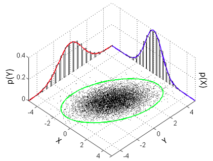
JAGS. The model that a classical Pearson’s correlation test assumes is that the data follows a bivariate normal distribution. That is, if we have a list $x$ of pairs of data points $[[x_{1,1},x_{1,2}],[x_{2,1},x_{2,2}],[x_{3,1},x_{3,2}],…]$ then the $x_{i,1} \text{s}$ and the $x_{i,2} \text{s}$ are each assumed to be normally distributed with a possible linear dependency between them. This dependency is quantified by the correlation parameter $\rho$ which is what we want to estimate in a correlation analysis. A good visualization of a bivariate normal distribution with $\rho = 0.3$ can be found on the
the wikipedia page on the multivariate normal distribution :
In
part one and
part two of Modeling Match Results in La Liga Using a Hierarchical Bayesian Poisson Model I developed a model for the number of goals in football matches from five seasons of La Liga, the premier Spanish football league. I’m now reasonably happy with the model and want to use it to rank the teams in La Liga and to predict the outcome of future matches!
Ranking the Teams of La Liga
We’ll start by ranking the teams of La Liga using the estimated skill parameters from the 2012/2013 season. The values of the skill parameters are difficult to interpret as they are relative to the skill of the team that had its skill parameter “anchored” at zero. To put them on a more interpretable scale I’ll first zero center the skill parameters by subtracting the mean skill of all teams, I then add the home baseline and exponentiate the resulting values. These rescaled skill parameters are now on the scale of expected number of goals when playing home team. Below is a caterpillar plot of the median of the rescaled skill parameters together with the 68 % and 95 % credible intervals. The plot is ordered according to the median skill and thus also gives the ranking of the teams.
# The ranking of the teams for the 2012/13 season.
team_skill <- ms3[, str_detect(string = colnames(ms3), "skill\\[5,")]
team_skill <- (team_skill - rowMeans(team_skill)) + ms3[, "home_baseline[5]"]
team_skill <- exp(team_skill)
colnames(team_skill) <- teams
team_skill <- team_skill[, order(colMeans(team_skill), decreasing = T)]
par(mar = c(2, 0.7, 0.7, 0.7), xaxs = "i")
caterplot(team_skill, labels.loc = "above", val.lim = c(0.7, 3.8))
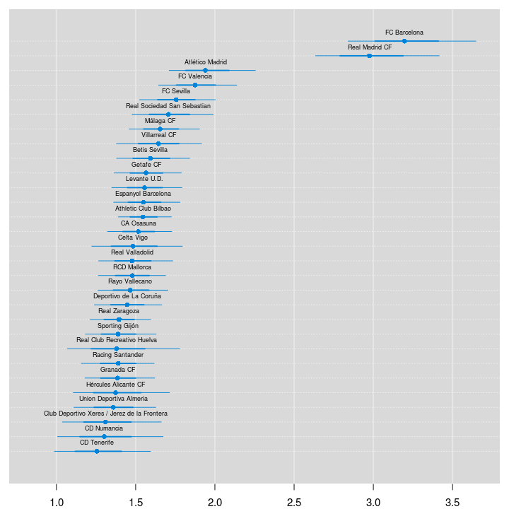
Two teams are clearly ahead of the rest, FC Barcelona and Real Madrid CF. Let’s look at the credible difference between the two teams.
One month ago I went to UseR 2013 in Albacete, Spain wich was a great conference featuring 33° C and many interesting presentations. Surpisingly CogSci 2013 in Berlin, which I attended this week, was even warmer, outside it is currenly 36° C! There were also many interesting presentations at CogSci 2013 with some of the highlights being:
The symposia on Music Cognition inlcuding a talk by Edward Large on how to model pitch and harmony perception using dynamical systems.
In
the last blog post I showed my initial attempt at modeling football results in La Liga using a Bayesian Poission model, but there was one glaring problem with the model; it did not consider the advantage of being the home team. In this post I will show how to fix this! I will also show a way to deal with the fact that the dataset covers many La Liga seasons and that teams might differ in skill between seasons.
Modeling Match Results: Iteration 2
The only change to the model needed to account for the home advantage is to split the baseline into two components, a home baseline and an away baseline. The following JAGS model implements this change by splitting baseline into home_baseline and away_baseline.
# model 2
m2_string <- "model {
for(i in 1:n_games) {
  HomeGoals[i] ~ dpois(lambda_home[HomeTeam[i],AwayTeam[i]])
  AwayGoals[i] ~ dpois(lambda_away[HomeTeam[i],AwayTeam[i]])
}

for(home_i in 1:n_teams) {
  for(away_i in 1:n_teams) {
    lambda_home[home_i, away_i] <- exp( home_baseline + skill[home_i] - skill[away_i])
    lambda_away[home_i, away_i] <- exp( away_baseline + skill[away_i] - skill[home_i])
  }
}

skill[1] <- 0
for(j in 2:n_teams) {
  skill[j] ~ dnorm(group_skill, group_tau)
}

group_skill ~ dnorm(0, 0.0625)
group_tau <- 1/pow(group_sigma, 2)
group_sigma ~ dunif(0, 3)

home_baseline ~ dnorm(0, 0.0625)
away_baseline ~ dnorm(0, 0.0625)
}"
Another cup of coffee while we run the MCMC simulation…
Update: This series of posts are now also available as a technical report:
Bååth, R. (2015), Modeling Match Results in Soccer using a Hierarchical Bayesian Poisson Model. LUCS Minor, 18. (ISSN 1104-1609) (
pdf)
This is a slightly modified version of my submission to the
UseR 2013 Data Analysis Contest which I had the fortune of winning :) The purpose of the contest was to do something interesting with a dataset consisting of the match results from the last five seasons of La Liga, the premium Spanish football (aka soccer) league. In total there were 1900 rows in the dataset each with information regarding which was the home and away team, what these teams scored and what season it was. I decided to develop a Bayesian model of the distribution of the end scores. Here we go…
Ok, first I should come clean and admit that I know nothing about football. Sure, I’ve watched Sweden loose to Germany in the World Cup a couple of times, but that’s it. Never the less, here I will show an attempt to to model the goal outcomes in the La Liga data set provided as part of the UseR 2013 data analysis contest. My goal is not only to model the outcomes of matches in the data set but also to be able to (a) calculate the odds for possible goal outcomes of future matches and (b) to produce a credible ranking of the teams. The model I will be developing is a Bayesian hierarchical model where the goal outcomes will be assumed to be distributed according to a Poisson distribution. I will focus more on showing all the cool things you can easily calculate in R when you have a fully specified Bayesian Model and focus less on model comparison and trying to find the model with highest predictive accuracy (even though I believe my model is pretty good). I really would like to see somebody try to do a similar analysis in SPSS (which most people uses in my field, psychology). It would be a pain!
This post assumes some familiarity with Bayesian modeling and Markov chain Monte Carlo. If you’re not into Bayesian statistics you’re missing out on something really great and a good way to get started is by reading the excellent
Doing Bayesian Data Analysis by John Kruschke. The tools I will be using is R (of course) with the model implemented in
JAGS called from R using the
rjags package. For plotting the result of the MCMC samples generated by JAGS I’ll use the
coda package, the
mcmcplots package, and the plotPost function courtesy of
John Kruschke. For data manipulation I used the
plyr and
stringr packages and for general plotting I used
ggplot2. This report was written in
Rstudio using
knitr and
xtable.
I start by loading libraries, reading in the data and preprocessing it for JAGS. The last 50 matches have unknown outcomes and I create a new data frame d holding only matches with known outcomes. I will come back to the unknown outcomes later when it is time to use my model for prediction.
I had a great time at useR 2013 in Albacete, Spain. The food was great, the people were fun and the weather was hot. A pleasant surprise was that I won the useR data analysis contest with my submission “Modeling Match Results in La Liga Using a Hierarchical Bayesian Poisson Model.” It was a fun exercise modeling football scores and I might write a post about it later, for now you can download my original submission here if you’re interested.
There are different ways of specifying and running Bayesian models from within R. Here I will compare three different methods, two that relies on an external program and one that only relies on R. I won’t go into much detail about the differences in syntax, the idea is more to give a gist about how the different modeling languages look and feel. The model I will be implementing assumes a normal distribution with fairly wide priors:
$$y_i \sim \text{Normal}(\mu,\sigma)$$
$$\mu \sim \text{Normal}(0,100)$$
$$\sigma \sim \text{LogNormal}(0,4)$$
Let’s start by generating some normally distributed data to use as example data in the models.
set.seed(1337)
y <- rnorm(n = 20, mean = 10, sd = 5)
mean(y)
## [1] 12.72
## [1] 5.762
Method 1: JAGS
JAGS (Just Another Gibbs Sampler) is a program that accepts a model string written in an R-like syntax and that compiles and generate MCMC samples from this model using Gibbs sampling. As in
BUGS, the program that inspired JAGS, the exact sampling procedure is chosen by an expert system depending on how your model looks. JAGS is conveniently called from R using the
rjags package and John Myles White has written
a nice introduction to using JAGS and rjags. I’ve seen it recommended to put the JAGS model specification into a separate file but I find it more convenient to put everything together in one .R file by using the textConnection function to avoid having to save the model string to a separate file. Now, the following R code specifies and runs the model above for 20000 MCMC samples:
library(rjags)

# The model specification
model_string <- "model{
  for(i in 1:length(y)) {
    y[i] ~ dnorm(mu, tau)
  }
  mu ~ dnorm(0, 0.0001)
  sigma ~ dlnorm(0, 0.0625)
  tau <- 1 / pow(sigma, 2)
}"

# Running the model
model <- jags.model(textConnection(model_string), data = list(y = y), n.chains = 3, n.adapt= 10000)
update(model, 10000); # Burnin for 10000 samples
mcmc_samples <- coda.samples(model, variable.names=c("mu", "sigma"), n.iter=20000)