Hello stranger, and welcome! 👋😊
I'm Rasmus Bååth, data scientist, engineering manager, father, husband, tinkerer,
tweaker, coffee brewer, tea steeper, and, occasionally, publisher of stuff I find
interesting down below👇
Everybody loves speed comparisons! Is R faster than Python? Is dplyr faster than data.table? Is STAN faster than JAGS? It has been said that speed comparisons are utterly meaningless, and in general I agree, especially when you are comparing apples and oranges which is what I’m going to do here. I’m going to compare a couple of alternatives to lm(), that can be used to run linear regressions in R, but that are more general than lm(). One reason for doing this was to see how much performance you’d loose if you would use one of these tools to run a linear regression (even if you could have used lm()). But as speed comparisons are utterly meaningless, my main reason for blogging about this is just to highlight a couple of tools you can use when you grown out of lm(). The speed comparison was just to lure you in. Let’s run!

For the second year round I and
Ullrika Sahlin arranged the mini-conference Bayes@Lund, with the aim of bringing together researchers in the south of Sweden working with Bayesian methods. This year the committee was also beefed up by
Paul Caplat and
Krzysztof Podgorski. What originally made me and Ullrika start this get-together is our feeling that Lund University is lagging behind with regards to Bayesian methods (we don’t have a single introductory course on Bayes stats!) and that we need a venue where people doing Bayes can meet and discuss what cool stuff they are working on. And so, last Tuesday, over 60 researchers got together to listen to twelve interesting talks, discuss, and (not least) fika. Here follows some highlights from Bayes@Lund 2015.

“Behind every great point estimate stands a minimized loss function.” – Me, just now
This is a continuation of Probable Points and Credible Intervals, a series of posts on Bayesian point and interval estimates. In
Part 1 we looked at these estimates as graphical summaries, useful when it’s difficult to plot the whole posterior in good way. Here I’ll instead look at points and intervals from a decision theoretical perspective, in my opinion the conceptually cleanest way of characterizing what these constructs are.
If you don’t know that much about Bayesian decision theory, just chillax. When doing Bayesian data analysis you get it
“pretty much for free” as esteemed statistician Andrew Gelman puts it. He then adds that it’s “not quite right because it can take effort to define a reasonable utility function.” Well, perhaps not free, but it is still relatively straight forward! I will use a toy problem to illustrate how Bayesian decision theory can be used to produce point estimates and intervals. The problem is this: Our favorite droid has gone missing and we desperately want to find him!

Peter Norvig, the director of research at Google, wrote a nice essay on
How to Write a Spelling Corrector a couple of years ago. That essay explains and implements a simple but effective spelling correction function in just 21 lines of Python. Highly recommended reading! I was wondering how many lines it would take to write something similar in base R. Turns out you can do it in (at least) two pretty obfuscated lines:
sorted_words <- names(sort(table(strsplit(tolower(paste(readLines("https://www.norvig.com/big.txt"), collapse = " ")), "[^a-z]+")), decreasing = TRUE))
correct <- function(word) { c(sorted_words[ adist(word, sorted_words) <= min(adist(word, sorted_words), 2)], word)[1] }
While not working exactly as Norvig’s version it should result in similar spelling corrections:
## [1] "piece"
## [1] "of"
## [1] "cake"

So let’s deobfuscate the two-liner slightly (however, the code below might not make sense if you don’t read
Norvig’s essay first):
Making a slight digression from last month’s
Probable Points and Credible Intervals here is how to summarize a 2D posterior density using a highest density ellipse. This is a straight forward extension of the highest density interval to the situation where you have a two-dimensional posterior (say, represented as a two column matrix of samples) and you want to visualize what region, containing a given proportion of the probability, that has the most probable parameter combinations. So let’s first have a look at a fictional 2D posterior by using a simple scatter plot:

Whoa… that’s some serious over-plotting and it’s hard to see what’s going on. Sure, the bulk of the posterior is somewhere in that black hole, but where exactly and how much of it?
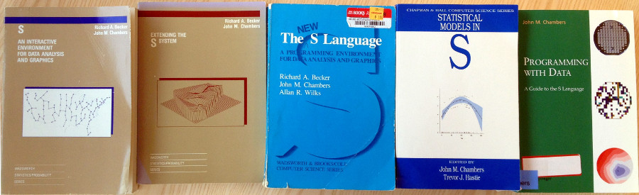
Why R? Because S!
R is the open source implementation (and a pun!) of S, a language for statistical computing that was developed at Bell Labs in the late 1970s. After that, the implementation of S underwent a number of major revisions documented in a series of seminal books, often just referred to by the color of their cover: The Brown Book, the Blue Book, the White Book and the Green Book. To satisfy my techno-historical lusts I recently acquired all these books and I though I would share some tidbits from them, highlighting how S (and thus R) developed into what we today love and cherish. But first, here are the books in chronological order from left to right:
After having broken the Bayesian eggs and prepared your model in your statistical kitchen the main dish is the posterior. The posterior is the posterior is the posterior, given the model and the data it contains all the information you need and anything else will be a little bit less nourishing. However, taking in the posterior in one gulp can be a bit difficult, in all but the most simple cases it will be multidimensional and difficult to plot. But even if it is one-dimensional and you could plot it (as, say, a density plot) that does not necessary mean that it is easy to see what’s going on.
One way of getting around this is to take a bite at a time and look at summaries of the marginal posteriors of the variables of interest, the two most common type of summaries being point estimates and credible intervals (an interval that covers a certain percentage of the probability distribution). Here one is faced with a choice, which of the many ways of constructing point estimates and credible intervals to choose? This is a perfectly good question that can be given an unhelpful answer (with a predictable follow-up question):
- That depends on your loss function.
- So which loss function should I use?
Big data is all the rage, but sometimes you don’t have big data. Sometimes you don’t even have average size data. Sometimes you only have eleven unique socks:
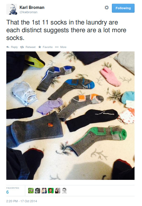
Karl Broman is here putting forward a very interesting problem. Interesting, not only because it involves socks, but because it involves what I would like to call Tiny Data™. The problem is this: Given the Tiny dataset of eleven unique socks, how many socks does Karl Broman have in his laundry in total?
If we had Big Data we might have been able to use some clever machine learning algorithm to solve this problem such as bootstrap aggregated neural networks. But we don’t have Big Data, we have Tiny Data. We can’t pull ourselves up by our bootstraps because we only have socks (eleven to be precise). Instead we will have to build a statistical model that includes a lot more problem specific information. Let’s do that!
As the normal distribution is sort of the default choice when modeling continuous data (but not necessarily the best choice), the Poisson distribution is the default when modeling counts of events. Indeed, when all you know is the number of events during a certain period it is hard to think of any other distribution, whether you are modeling the
number of deaths in the Prussian army due to horse kicks or the
numer of goals scored in a football game. Like the t.test in R there is also a poisson.test that takes one or two samples of counts and spits out a p-value. But what if you have some counts, but don’t significantly feel like testing a null hypothesis? Stay tuned!

I was lucky enough to be presenting at
the 14th International Conference on Music Perception and Cognition in Seoul, South Korea, last week. It was a very inspiring conference and I really like South Korea (especially the amazing food…). My presentation was on the topic of subjective rhythmization, a fascinating auditory illusion. See below for my
presentation slides and for a short conference paper that was published in the proceedings of the conference:
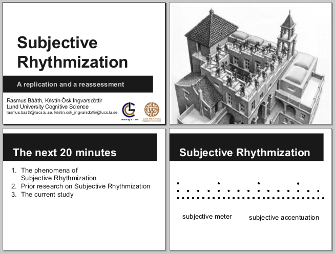
Bååth, R., Ingvarsdóttir, K. O. (2014) Subjective Rhythmization: A Replication And an Extension. Proceedings of the 13th International Conference on Music Perception and Cognition in Seoul, South Korea.
pdf of full paper